Week 3 - Solving second order ODEs

Aim :

Solving the second order differential equation for the simple pendulum motion using MATLAB

Objective:

To write the program that will solve the following ODE equation. Also create the animation video that will show the pendulum motion with respect to time.

ODE EQUATION:

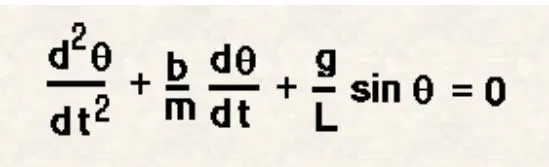
Other initial conditions:

Gravity(g)=9.81m/s^2

Damping coefficient(b)=0.05

Mass of the ball(m)=1kg

Length of the pendulum(l)=1m

Time of motion=0-20sec

Initial velocity=3m/s

Initial displacement=0

Introduction:

ODE is used to describe the transient behavior of a system. A simple example is a pendulum

The way the pendulum moves depends on the Newtons second law. When this law is written down, we get a second order Ordinary Differential Equation that describes the position of the "ball" w.r.t time.

Simple Pendulum - Newtonian

Now let's look at another famous example, 'Simple Pendulum (Single Pendulum)'. Governing Law is same as other dynamic system saying "Total Force being applied to a moving body represents the motion of the body". Basic format is derived from F = ma. The only difference is that Pendulum is for rotational motion whereas F=ma is for linear movement, but the basic concept is same.

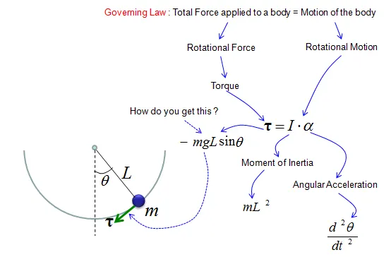
Fig- simple pendulum equation derivation basics

Similarly, there are hundreds of ODEs that describe key phenomena and if you have the ability to solve these equations then you will be able to simulate any of these systems.

Program:

clear all 
close all
clc
 
%solving the ODE ofsimple pendulum motion
%input fixed paramters
 
%damping coefficient 
b=0.05;
%gravity(m/s^2)
g=9.81;
%length in m
l=1;
%mass in kg
m=1;
 
 
%initial condition
theta_0=[0;3];
 
%time 
tspan=linspace(0,20,300);
 
%solving 
[t,results]= ode45(@(t,theta) ode_func(t,theta,b,g,l,m),tspan,theta_0)
 
 
%plotting
figure(1)
plot(t,results(:,1),'--')
hold on
plot(t,results(:,2))
xlabel('time')
ylabel('velocity & displacement')
 
ct=1;
for i=1:length(results(:,1))
    x0=0;
    y0=0;
    
    x1=l*sin(results(i,1));
    y1=-l*cos(results(i,1));
    
    figure(2)
    plot([-1 1],[0,0],'-.','color',[0 0 0.5]);
    hold on;
    plot([x0 x1],[y0 y1],'linewidth',4,'color','r');
    hold on;
    plot(x1,y1,'o','markers',20,'markerfacecolor','g');
    axis([-2 2 -1.5 1]);
    pause(0.1);
    hold off;
    M(ct)=getframe(gcf);
    ct=ct+1;
end
movie(M)
videofile=VideoWriter('ode_simple_pendulum.avi','Uncompressed AVI');
open(videofile)
writeVideo(videofile,M)
close(videofile)

Explanation:

The program is started with the defining the initial parameters required in the equation like gravity , damping coefficient, mass and length.

The above parameter is the array with first being the displacement and the other being the velocity as the initial condition for the pendulum.

tspan=linspace(0,20,300);

The time span is the time for the rotation of the pendulum. Here we have used the linspace command with values of 300, so that between 0-20 there are total of 300 values with constant difference between two consecutive values.

• Function and calling the function:

To solve the second order differential equation, the equation is converted to first order equation. This is achieved by creating the additional function in which the second order in converted to first order equation by simply assigning the variables to second order. The function syntax is as follow

Here ,

The b,g,l,m are inputs of the function and the ode_func is the name of the function that will be used in calling in the main program

d(theta1)/dt=theta2

Further the equation is simplified into series of single order ODE. Lastly the values of the both single order are represented in the form of array as dtheta1_dt; dtheta2_dt.

• Ode solver :

Ode45 is the by default solver in the MATLAB that have the inputs as t, theta. Its syntax is as follows

[t,results]= ode45(@(t,theta) ode_func(t,theta,b,g,l,m),tspan,theta_0)

Tspan and theta_0 are the initial conditions for the equation. The above syntax solve the equation and gives the all the values of the displacement and velocity till 300 iterations.

• Plotting the graph:

The graph is plotted between the time and velocity also displacement. So in order to accommodate the both the plot is same figure we have used the hold on command.

plot(t,results(:,1),'--')

The above syntax plot the graph for the displacement vs time. Since we have written results(:,1) , first column in the results is the displacement. Also the displacement line is denoted by the dashed line “--”.

plot(t,results(:,2))

the above syntax plot the graph for velocity vs time. Later on the both the axis is labelled accordingly.

• Loop for the animation:

Ct=1

This is the counter command to create the figure of the plot and to count the number of event inside the loop. This figure window initially is set to 1 value, which will be incremented at the end to get the continuous frame.

Inside the loop the initial and final position of the pendulum arm is defined as x0,y0,x1,y1 respectively.

Plotting and animation video:

Here the plot is started with naming the plot as figure(2)

plot([-1 1],[0,0],'-.','color',[0 0 0.5]);

The above syntax gives the horizontal base line as dashed and dotted. Here also we are using the hold on command to accommodate all the lines in the same figure .

plot([x0 x1],[y0 y1],'linewidth',4,'color','r');

the above syntax plot the pendulum arm initial and final position. The x1,y1 is an array with the total values of 300. The width of the line is set to 4 size and the color as red.

plot(x1,y1,'o','markers',20,'markerfacecolor','g');

Since pendulum mass is a single point , it will have only one coordinate as x1,y1. For pendulum we have used the marker to set the defined size and colour.

Then the axis is set and the pause (0.1) is used to pause the frame 0.1 sec between two consecutive position of the pendulum.

The all the counted frame is stored in the M (gcf=get current frame). The counter is then incremented by 1 for continuous frames.

Lastly all the syntax are used to create the movie of the pendulum arm movement with respect to time.

Results:

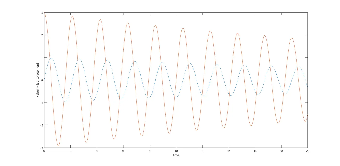
Fig- damped motion of the pendulum (velocity & displacement vs time)

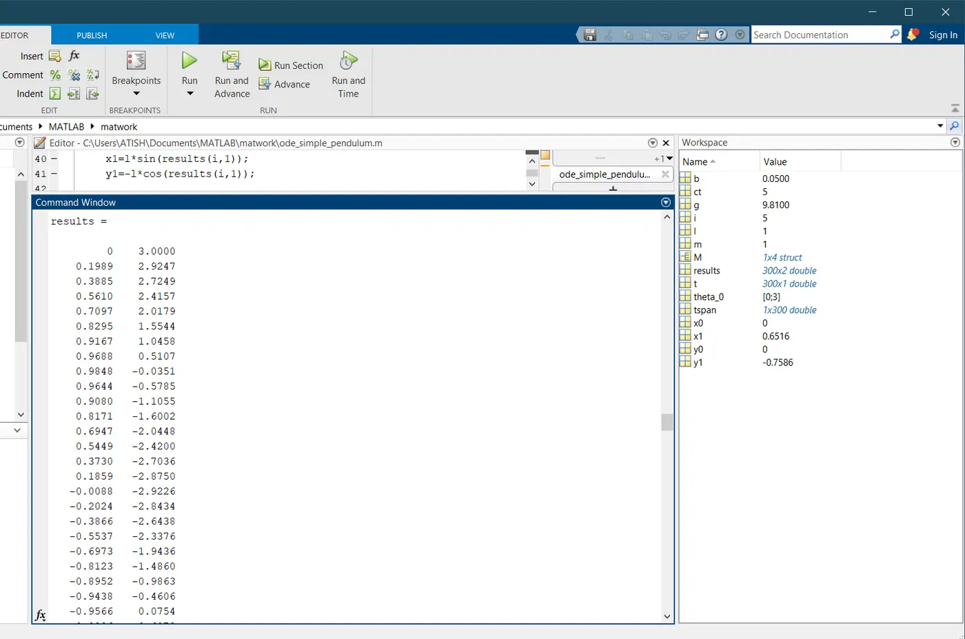
Fig - Result array along with workspace showing final values

Conclusions:

The plot for the displacement and velocity against the time shows the damping motion since we have used damping coefficient as 0.05. The animation for the pendulum displacement as function of time is successfully created.

Link for the video: https://www.youtube.com/watch?v=UIA665aRyPg