Week 8- Moving zones approach in Fluent

Moving zones approach in Fluent

Aim:

• What are the approaches by which you would model moving zones?
• Which approaches would you use to model unsteady phenomena?
• Simulate rotary motion for the geometry given

1. Plot the velocity profile of the fluid motion.

Moving zone approaches:

The solution of flows in moving reference frames requires the use of moving cell zones. This cell zone motion is interpreted as the motion of a reference frame to which the cell zone is attached. With this capability,

A wide variety of problems that involve moving parts can be set up and solved using FLUENT.

Overview of Moving Zones Approaches

• flow in a (single) rotating frame
• Flow in multiple rotating and/or translating reference frames.

So in order to Model Moving Zones approaches Fluent has these set of Categories (Example - In turbo machinery applications where rotor and stator blades are in close proximity (and hence rotor-stator interaction is important)).

• Single reference of frame (SRF) model.
• The multiple reference frame (MRF) model
• the mixing plane model
• the sliding mesh model

Single Reference of Frame (SRF):

Many problems permit the entire computational domain to be referred to as a single rotating reference frame (hence the name SRF modeling). In such cases, the equations given above are solved in all fluid cell zones. Steady-state solutions are possible in SRF models provided suitable boundary conditions are prescribed. But the wall boundaries must meet certain requirements, as mentioned below:

• The wall which is moving with the reference frame may assume any shape.
• Boundaries which are stationary should be the surface of revolution about axis of rotation.

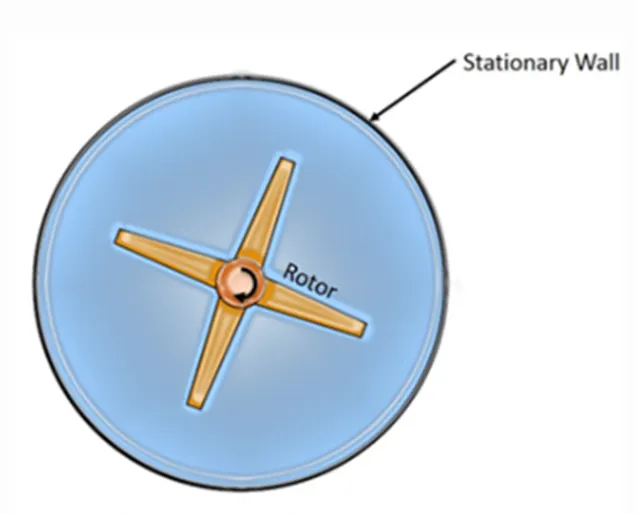
An example where SRF approach can be applied is shown above. In the example, the domain contains a rotor which is moving at certain angular velocity and a stationary wall. In this case the problem can be solved using SRF approach, since no stationary walls are present inside the domain and the outer stationary wall is surface of revolution and meets the above criteria. But when the problem involves multiple rotating parts or stationary components (like guide vanes in turbines) that are not the surface of revolution, the SRF modelling approach fails. Thus a different approach has to be adopted to solve such kind of problems by breaking the domain into stationary zone and rotating zone with interface separating them. Based on the manner in which interface is treated two approaches are defined namely

Multiple reference frame (MRF) model:

The MRF model is the simplest of the two approaches for multiple zones. It is a steady-state approximation in which individual cell zones move at different rotational and/or translational speeds. The flow in each moving cell zone is solved using the moving reference frame equations. If the zone is stationary {tex}(\omega = 0){/tex}, the stationary equations are used i.e., moving reference frame equations are solved in rotational zone and stationary equations are solved in stationary zone and the information is exchanged at the interface. The properties of the flow at the interface between the stationary and rotating zones is directly translated in MRF. In MRF approach there is no relative motion between moving zone with respect to the adjacent zone, the grid is fixed for computation. This is analogous to freezing the motion of the moving part in a specific position and observing the instantaneous flow field with the rotor in that position and hence, the MRF is often referred to as the "frozen rotor approach."

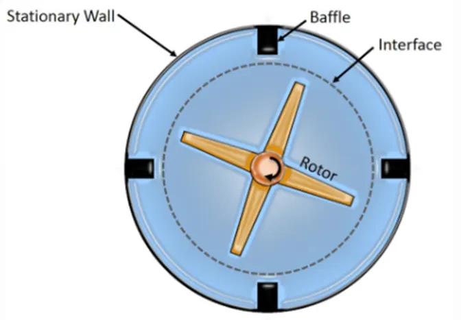
An example that illustrates the MRF approach is shown with an above (image). In the image apart from the rotor and stationary walls there are stationary baffles present inside the fluid zone. Thus an interface is defined which is a surface of revolution about the rotor axis to distinguish between stationary and rotating zone. MRF model should be used when the flow is not complicated and if the interaction between rotor and stator in a turbine stage is weak. With a MRF simulation rotating wakes, secondary flows, leading edge pressure increases etc.will always stay in exactly the same positions. This makes the simulation very dependent on exactly how the rotors and the stators are positioned. Usually MRF model is used to calculate flow field that can be used as initial condition for sliding mesh calculation.

Problem set-up:

• The meshed model is imported into ANSYS FLUENT.
• Under the general conditions, Pressure based solver is used. A steady state analysis is performed. Generally with Moving Reference Frame, steady state studies are conducted. . 2d planar analysis is done.
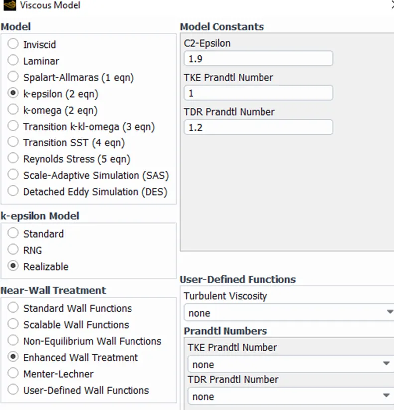
• Under the models tab, turbulence modelling is performed. Both k omega SST and K epsilon model gives satisfactory results, but in this project, RNG K -epsilon model is used for analysis.
• The material for analysis is air.
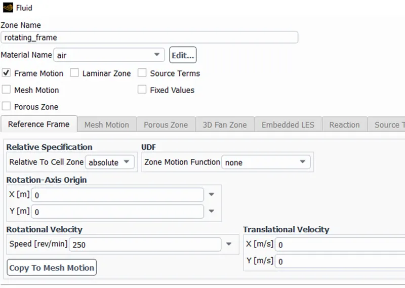
• In the cell zones, under the zones, rotating frame is enabled. Frame motion box is checked.
• In the rotation axis, the origin is set to (0,0) which is perfectly fine for this model.
• The angular velocity for this model is 250 rpm. There are two ways, either the value of the angular velocity is changed to radian per seconds or the units of the angular velocity is changed to rpm in fluent.

Viscous Model:

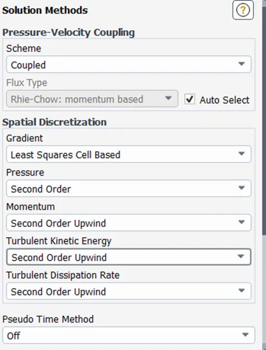
Solution Method:

Cell Zone Conditions:

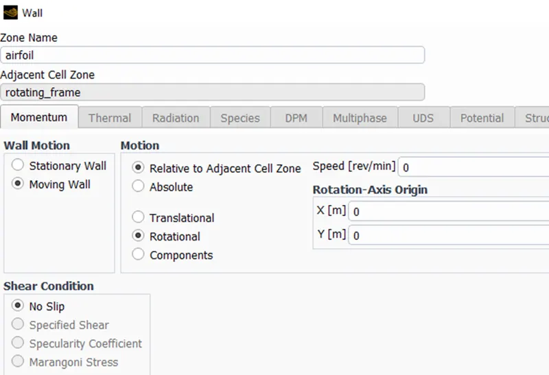
Boundary Condition for Airfoil:

Results:

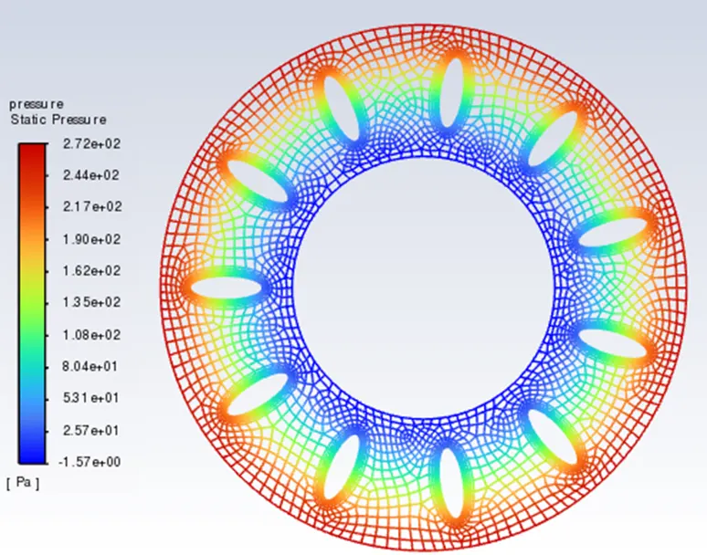
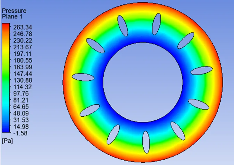
Static pressure:

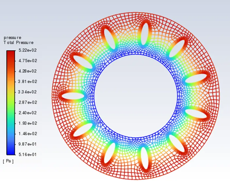
Total pressure:

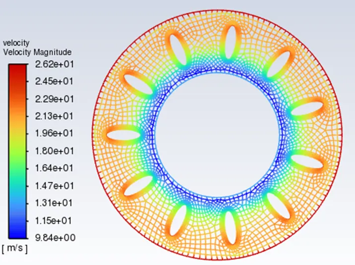
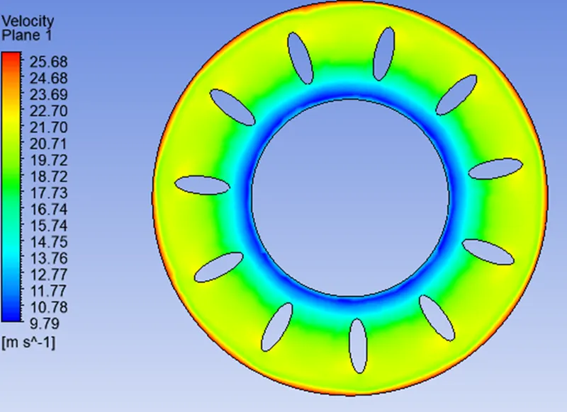
Velocity contour:

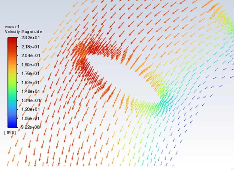
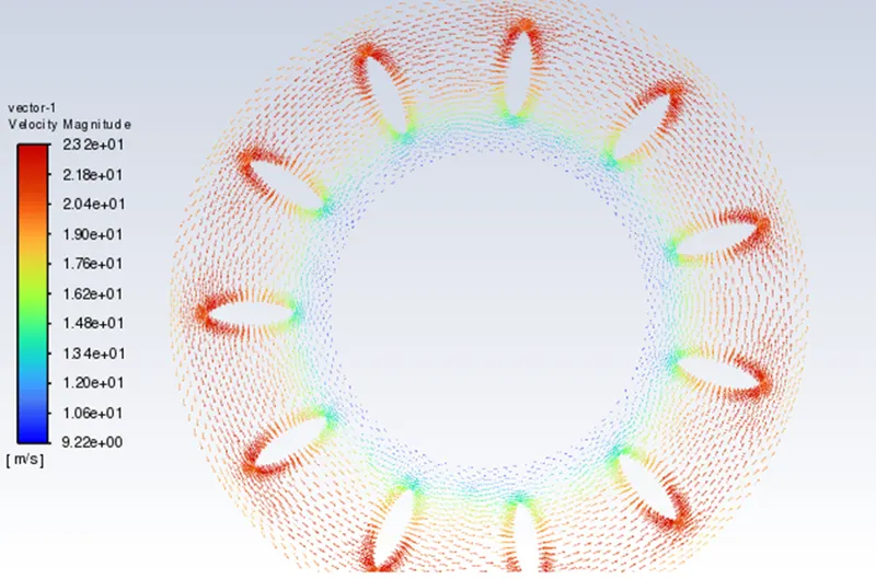
Vector velocity:

Conclusion:

From the velocity contours and the velocity vectors, the direction of the flow can be visualized. The velocity is lower in the inner frame, whereas as we move towards the outer frame, the velocity increases.