Week 7 - Simulation of a 1D Super-sonic nozzle flow simulation using Macormack Method

Simulation of a 1D Super-sonic nozzle flow simulation using Macormack Method

Aim:

In this challenge you are going to simulate the isentropic flow through a quasi 1D subsonic-supersonic nozzle. You will derive both the conservation and non-conservation forms of the governing equations and sovle them using the MacCormack's technique. You need to determine the steady-state temperature distribution for the flow-field variables and investigate the difference between the two forms of governing equations by comparing their solutions.

You need to show the following plots inside your report
1. Steady-state distribution of primitive variables inside the nozzle
2. Time-wise variation of the primitive variables
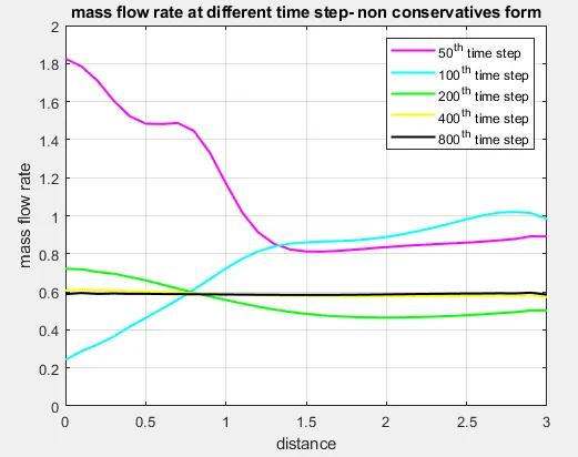
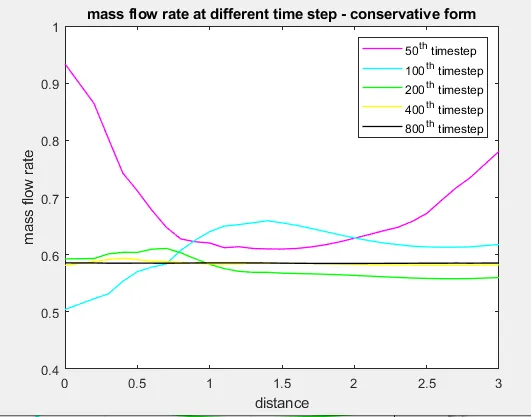
3. Variation of Mass flow rate distribution inside the nozzle at different time steps during the time-marching process
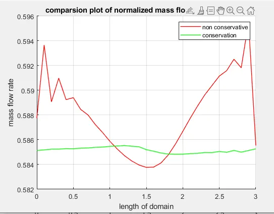
4. Comparison of Normalized mass flow rate distributions of both forms

Theory:

Any numerical solution of isentropic flow though a quasi 1d subsonic –supersonic nozzle is unreasonable, while analytical solution exists for these kind of problems.

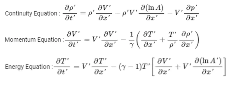
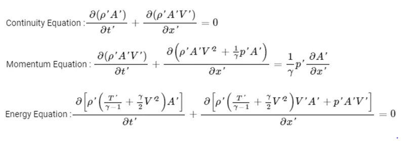
Governing equations are marched in terms of PDE for both forms in order to use time marching solution for the problem. These forms represent in numerical aspect only, if we analytical all the methods are same.

Non conservative form:

Conservative form:

Non dimensional quantities:

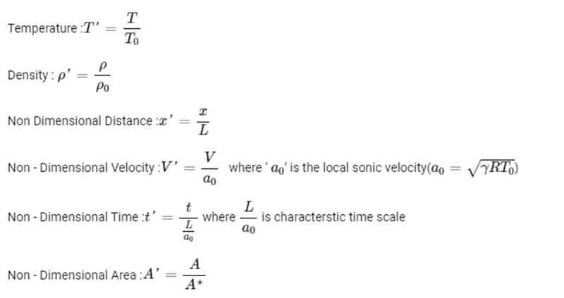
Also as part of the problem setup we represent quantities in terms of non-dimensional quantities.

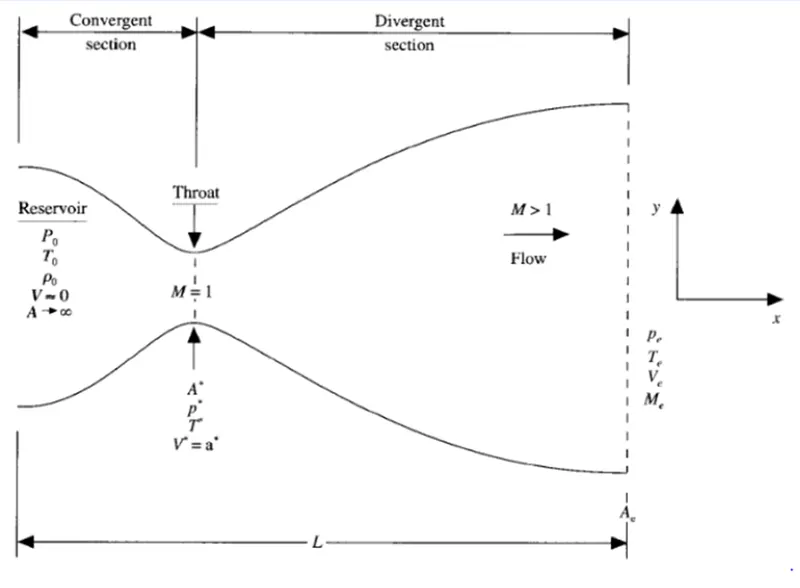
Nozzle diagram with section:

Since the problem setup is 1D, we consider only distribution in x-axis. Here nozzle can be split into two section

• Convergent section
• Divergent section

McCormack method:

To discretize the numerical solution we use the technique called McCormack method. The McCormack method is a variation of the two-step Lax-Wendroff scheme but is much simpler in application.

The application of McCormack method proceeds in two steps, a predictor step which is followed by a corrector step.

• Predictor step: in the predictor step, a “provisional” value of U at time level n+1 (denoted by u_i­ⁿ⁺¹) is estimated obtained by replacing the spatial and temporal derivatives in the previous first order equation using forward difference scheme. Δt is used for time step.
• Corrector step: in the corrector step, the predicted value u_i­ⁿ⁺¹ is corrected according to the equation. Note that the corrector step uses backward difference scheme for spatial derivative. The time-step used in the corrector step Δt/2 in contrast to the Δt used in the predictor step.

In order for the code to be modular, program is split into three section. They are

1. Main program of quasi 1D subsonic-supersonic nozzle.

Two functions namely

• Non-conservative form
• Conservative form

Let f(x) is the equation to be solved. Then the following steps are followed.

• Initial profile:

Before the calculation, the initial profile for all the flow field variables which are velocity, density and temperature has to be determined. These are guess values but should be specified with more awareness on the problem.

• Predictor step:

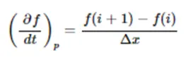
• Solution update:

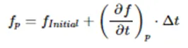
F_p = flow field variables calculated after the predictor step.

F_initial = flow field variables in the initial step.

Δt = time step size.

• Corrector step:

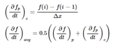
• Final solution update:

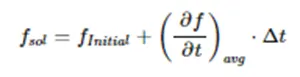
F_(sol) = final solution of the flow field variables for the first time step.

main matlab code:

clear all
close all
clc

n = 31;
gamma = 1.4;
x = linspace(0,3,n);
dx = x(2) - x(1);
nt = 1400;
cfl = 0.5;

% function of Non conservative form
tic;
[mfr_nc,p_nc,M_nc,rho_nc,v_nc,T_nc,rho_throat_nc,v_throat_nc,T_throat_nc,mfr_throat_nc,p_throat_nc,M_throat_nc]= non_conservative_form(x,dx,n,gamma,nt,cfl)
time_elapsed_nc=toc;
fprintf('time elasped for non conservative form %0.4f',time_elapsed_nc)
hold on

% plotting
% time variation of properties at throat area in non conservative form
figure(2)

% density
subplot(4,1,1)
plot(linspace(1,nt,nt),rho_throat_nc,'Color','m')
xlabel('time stpe')
ylabel('density')
legend({'dendity at throat'})
axis([0 1400 0 1.3]);
title('time step variation at throat area- non conservative form')

% temperature
subplot(4,1,2)
plot(linspace(1,nt,nt),T_throat_nc,'Color','c')
xlabel('time stpe')
ylabel('temperature')
legend({'temperature at throat'})
axis([0 1400 0.6 1]);
title('time step variation at throat area- non conservative form')

% pressure
subplot(4,1,3)
plot(linspace(1,nt,nt),p_throat_nc,'Color','g')
xlabel('time stpe')
ylabel('pressure')
legend({'pressure at throat'})
axis([0 1400 0.4 1.1]);
title('time step variation at throat area- non conservative form')

% mach number
subplot(4,1,4)
plot(linspace(1,nt,nt),M_throat_nc,'Color','y')
xlabel('time stpe')
ylabel('mach number')
legend({'mach number at throat'})
axis([0 1400 0.6 1.4]);
title('time step variation at throat area- non conservative form')

% steady-state simulation primitves values for non conservatives form
figure(3)

% density
subplot(4,1,1)
plot(x,rho_nc,'Color','m')
xlabel('timesteps')
ylabel('density')
legend({'density'})
axis([0 3 0 1])
title('variation of flow rate distribustion- non conservation form')

% temperature
subplot(4,1,2)
plot(x,T_nc,'Color','c')
xlabel('timesteps')
ylabel('temperature')
legend({'temperature'})
axis([0 3 0 1])
title('variation of flow rate distribustion- non conservation form')

% preasure
subplot(4,1,3)
plot(x,p_nc,'Color','g')
xlabel('timesteps')
ylabel('preasure')
legend({'preasure'})
axis([0 3 0 1])
title('variation of flow rate distribustion- non conservation form')

% mach number
subplot(4,1,4)
plot(x,M_nc,'Color','y')
xlabel('timesteps')
ylabel('mach number')
legend({'mach number'})
axis([0 3 0 4])
title('variation of flow rate distribustion- non conservation form')

% function for conservative form
tic;
[mfr_c,p_c,M_c,rho_c,v_c,T_c,rho_throat_c,v_throat_c,T_throat_c,mfr_throat_c,p_throat_c,M_throat_c] = conservative_form(x,dx,n,gamma,nt,cfl)
time_elapsed_c= toc;
fprintf('time elapsed for conservative %0.4f',time_elapsed_c)

% poltting
% time variation of propertics at throat area conservation form

figure(5)
% density
subplot(4,1,1)
plot(rho_throat_c,'color','m')
xlabel('time step')
ylabel('density')
legend('density at throat')
axis([0 1400 0 1])
title('time step variation at throat area- conservation form')

% temperatre
subplot(4,1,2)
plot(T_throat_c,'color','c')
ylabel('temperature')
legend('temperature at throat')
axis([0 1400 0.6 1])

% pressure
subplot(4,1,3)
plot(p_throat_c,'color','g')
ylabel('pressure')
legend('pressure at throat')
axis([0 1400 0.2 0.8])

% mach number
subplot(4,1,4)
plot(M_throat_c,'color','y')
ylabel('mach number')
legend('mach number at throat')
axis([0 1400 0.6 1.4])

% steady state simlulation for prmitive values for conservative form
figure(6)
% density
subplot(4,1,1)
plot(x,rho_c,'color','m')
ylabel('density')
legend('density')
axis([0 3 0 1])
title('variation of flow rate distrbution - conservation form')

% temperature
subplot(4,1,2)
plot(x,T_c,'color','c')
ylabel('temperature')
legend('temperature')
axis([0 3 0 1])

% pressure
subplot(4,1,3)
plot(x,p_c,'color','g')
ylabel('pressure')
legend('pressure')
axis([0 3 0 1])

% mach number
subplot(4,1,4)
plot(x,M_c,'color','y')
ylabel('mach number')
legend('mach number')
axis([0 3 0 4])

% comparsion plot of normalized mass flow rate both forms
figure(7)
hold on
plot(x,mfr_nc,'r','LineWidth',1)
hold on
plot(x,mfr_c,'g','LineWidth',1)
hold on
grid on

legend('non conservative','conservation')
xlabel('length of domain')
ylabel('mass flow rate')
title('comparsion plot of normalized mass flow rate both forms')

Explanation:

• Input parameters are assigned for the variables x, dx, n, gamma, nt, and CFL.
• Non conservative and conservative forms are created as separate function with the necessary inputs which is detailed below this section.
• Tic, toc command is used for calculating the time elapsed between the function.
• Plotting is done for the following solutions.
  1. Time step variation at throat area of both forms.
  2. Variation of flow rate distribution of both forms.
  3. Comparison of normalized mass flow rate of both forms.
• Each plot is computed as subplot of four primitive variables such as density, temperature, pressure and Mach number at throat as well as convergent/divergent section.

Non-conservative form:

function [mfr_nc,p_nc,M_nc,rho_nc,v_nc,T_nc,rho_throat_nc,v_throat_nc,T_throat_nc,mfr_throat_nc,p_throat_nc,M_throat_nc]= non_conservative_form(x,dx,n,gamma,nt,cfl)

% initial boundary condition
rho_nc = 1-0.3146*x;
T_nc = 1-0.2341*x;
v_nc = (0.1+1.09*x).*T_nc.^0.5;

% area &throat profile
a = 1+2.2*(x - 1.5).^2;
throat = find(a==1);

% outer time loop
for k= 1:nt

% time step
dt = min(cfl.*dx./(sqrt(T_nc)+v_nc));

% old values
rho_old= rho_nc;
T_old= T_nc;
v_old= v_nc;

% predictor step
for j= 2:n-1

drhodx = (rho_nc(j+1)-rho_nc(j))/dx;
dvdx = (v_nc(j+1)-v_nc(j))/dx;
dTdx = (T_nc(j+1)-T_nc(j))/dx;
dlogadx = (log(a(j+1))-log(a(j)))/dx;

% continuity equation
drhodt_p(j)= - rho_nc(j) * dvdx - rho_nc(j) * v_nc(j) * dlogadx - v_nc(j) * drhodx;
% momentum equation
dvdt_p(j)= - v_nc(j) * dvdx - (1/gamma) * (dTdx + (T_nc(j)*drhodx/rho_nc(j)));
% energy equation
dTdt_p(j)= - v_nc(j) * dTdx -(gamma-1) * T_nc(j) * (dvdx + v_nc(j) * dlogadx);

% soluation update
rho_nc(j) = rho_nc(j) + drhodt_p(j)*dt;
v_nc(j) = v_nc(j) + dvdt_p(j)*dt;
T_nc(j) = T_nc(j) + dTdt_p(j)*dt;
end

% corrector step
for j= 2:n-1
drhodx = (rho_nc(j)-rho_nc(j-1))/dx;
dvdx = (v_nc(j)-v_nc(j-1))/dx;
dTdx = (T_nc(j)-T_nc(j-1))/dx;
dlogadx = (log(a(j))-log(a(j-1)))/dx;

% continuity equation
drhodt_c(j)= - rho_nc(j) * dvdx - rho_nc(j) * v_nc(j) * dlogadx - v_nc(j) * drhodx;
% momentum equation
dvdt_c(j)= - v_nc(j) * dvdx - (1/gamma) * (dTdx + (T_nc(j)*drhodx/rho_nc(j)));
% energy equation
dTdt_c(j)= - v_nc(j) * dTdx -(gamma-1) * T_nc(j) * (dvdx + v_nc(j) * dlogadx);
end

% compute average time dervative
drhodt = 0.5.*(drhodt_p + drhodt_c);
dvdt = 0.5.*(dvdt_p + dvdt_c);
dTdt = 0.5.*(dTdt_p + dTdt_c);

% final soluation update
for i= 2:n-1
rho_nc(i) = rho_old(i) + drhodt(i)*dt;
v_nc(i) = v_old(i) + dvdt(i)*dt;
T_nc(i) = T_old(i) + dTdt(i)*dt;
end

% boundary condition
% inlet
rho_nc(1) = 1;
v_nc(1) = 2*v_nc(2)-v_nc(3);
T_nc(1) = 1;
% outlet
rho_nc(n) = 2* rho_nc(n-1)- rho_nc(n-2);
v_nc(n) = 2* v_nc(n-1)- v_nc(n-2);
T_nc(n) = 2* T_nc(n-1)- T_nc(n-2);

% deifining massflow rate, pressure, mach number
mfr_nc = rho_nc.*a.*v_nc;
p_nc = rho_nc.*T_nc;
M_nc = (v_nc./sqrt(T_nc));

% calculating variable at throat point
rho_throat_nc(k) = rho_nc(throat);
T_throat_nc(k) = T_nc(throat);
v_throat_nc(k) = v_nc(throat);
mfr_throat_nc(k) = mfr_nc(throat);
p_throat_nc(k) = p_nc(throat);
M_throat_nc(k) = M_nc(throat);

% plotting
% comparsion of non dimensional mass flow rate at different time step
figure(1);
if k==50
plot(x,mfr_nc,'m','LineWidth',1.5)
hold on
elseif k==100
plot(x,mfr_nc,'c','LineWidth',1.5)
hold on
elseif k==200
plot(x,mfr_nc,'g','LineWidth',1.5)
hold on
elseif k==400
plot(x,mfr_nc,'y','LineWidth',1.5)
hold on
elseif k==800
plot(x,mfr_nc,'k','LineWidth',1.5)
hold on
end

% labelling
title('mass flow rate at different time step- non conservatives form')
xlabel('distance')
ylabel('mass flow rate')
legend({'50^t^h time step','100^t^h time step','200^t^h time step','400^t^h time step','800^t^h time step'})
axis([0 3 0 2])
grid on
end
end

Explanation:

• The purpose of the function is to calculated the values of mass flow rate, pressure, Mach number, density, velocity, temperature, density at throat, velocity at throat, temperature at throat, mass flow rate at throat, pressure at throat, Mach number at throat by the known equation for all the grid points.
• For this initial boundary conditions are established for density, temperature and velocity and profiles for calculating area and throat.
• Now outer time loop is computed for ‘for loop’ to calculate all the grid points for various formulas inside the loop.
• McCormack technique is used to solve the numerical solution of governing equation such as continuity, momentum and energy equation.
• The technique implies two methods are assigned within the ‘for loop’ individually for calculating values.
• The calculated values are averaged in the next step and updating the solution with old values.
• Boundary condition are applied within the ‘for loop’ and subsequently used for calculating the mass flow rate, Mach number and pressure and also calculating the values throated section.
• Finally plotting is done for distance(x) and mass flow rate for different time steps.

Conservative form:

function [mfr_C,p_C,M_C,rho_C,v_C,T_C,rho_throat_C,v_throat_C,T_throat_C,mfr_throat_C,p_throat_C,M_throat_] = Conservative_form(x,dx,n,gamma,nt,cfl)

% initial profile of density and temperature
for i=1:n

if (x(i)>=0 && x(i) <= 0.5)
rho_C (i)= 1;
T_C(i)= 1;
elseif (x(i)>=0.5 && x(i)<=1.5)
rho_C(i)= 1 - 0.366*(x(i)-0.5);
T_C(i)= 1 - 0.167*(x(i)-0.5);
elseif (x(i)>=1.5 && x(i)<=3)
rho_C(i)= 0.634 - 0.3879*(x(i)-1.5);
T_C(i)= 0.833 - 0.3507*(x(i)-1.5);
end
end

% area and throat profile
a= 1 + 2.2*(x - 1.5).^2;
throat = find(a==1);

% initial profile pressure and velocity
v_C = 0.59./(rho_C.*a);
p_C = rho_C.*T_C;

% calculating the initial soluation vectors
u1= rho_C.*a;
u2= rho_C.*a.*v_C;
u3= rho_C.*a.*(T_C./(gamma-1)) + ((gamma/2).*v_C.^2);

% outer time loop
for k= 1:nt

% time step control
dt = min (cfl.*dx./(sqrt(T_C) + v_C));

% old values
u1_old = u1;
u2_old = u2;
u3_old = u3;

% claculate the flux vector(f)
f1 = u2;
f2 = ((u2.^2)./u1) + ((gamma-1)/gamma) * (u3- (gamma/2)*((u2.^2)./u1));
f3 = ((gamma*u2.*u3)./u1) - (gamma*(gamma-1)*((u2.^3)./(2*u1.^2)));

% predictor
for j = 2:n-1

% sourse terms
j2(j) = (1/gamma)*rho_C(j)*T_C(j)*((a(j+1) - a(j))/dx);

% continuity equation
du1dt_p(j) = -((f1(j+1) - f1(j))/dx);

% momentum equation
du2dt_p(j) = -((f2(j+1) - f2(j))/dx) +j2(j);

% energy equation
du3dt_p(j) = -((f3(j+1) - f3(j))/dx);

% updateing new values
u1(j) = u1(j) + du1dt_p(j)*dt;
u2(j) = u2(j) + du2dt_p(j)*dt;
u3(j) = u3(j) + du3dt_p(j)*dt;
end

% updating flux vector
f1 = u2;
f2 = ((u2.^2)./u1) + ((gamma-1)/gamma)* (u3-((gamma*0.5*(u2.^2))./(u1)));
f3 = ((gamma*u2.*u3)./u1) - (gamma*0.5*(gamma-1)*(u2.^3)./(u1.^2));

% corrector method
for j=2:n-1

j2(j) = (1/gamma)*rho_C(j)*T_C(j)*((a(j) - a(j-1))/dx);

% continuity equation
du1dt_c(j) = -((f1(j) - f1(j-1))/dx);

% momentum equation
du2dt_c(j) = -((f2(j) - f2(j-1))/dx) +j2(j);

% energy equation
du3dt_c(j) = -((f3(j) - f3(j-1))/dx);
end

% compute average time dervative
du1dt_avg = 0.5*(du1dt_p + du1dt_c);
du2dt_avg = 0.5*(du2dt_p + du2dt_c);
du3dt_avg = 0.5*(du3dt_p + du3dt_c);

% finial soluaion update value
for i= 2:n-1
u1(i) = u1_old(i) + du1dt_avg(i)*dt;
u2(i) = u2_old(i) + du2dt_avg(i)*dt;
u3(i) = u3_old(i) + du3dt_avg(i)*dt;
end

% applying boundary conditions
% inlet
u1(1) = rho_C(1) * a(1);
u2(1) = 2*u2(2) - u2(3);
v_C(1) = u2(1)./u1(1);
u3(1) = u1(1)*((T_C(1)/(gamma-1))+((gamma/2)*(v_C(1)).^2));

% outlet
u1(n) = 2*u1(n-1) - u1(n-2);
u2(n) = 2*u2(n-1) - u2(n-2);
u3(n) = 2*u3(n-1) - u3(n-2);

% final primitive value update
rho_C = u1./a;
v_C = u2./u1;
T_C = (gamma-1)* ((u3./u1 - (gamma/2)*(v_C).^2));

% define mfr, pressure, mach number
mfr_C = rho_C.*a.*v_C;
p_C = rho_C.*T_C;
M_C = (v_C./sqrt(T_C));

% calculating different variables throat point
rho_throat_C(k)= rho_C(throat);
T_throat_C(k)= T_C(throat);
v_throat_C(k)= v_C(throat);
mfr_throat_C(k)= mfr_C(throat);
p_throat_C(k)= p_C(throat);
M_throat_(k)= M_C(throat);

% plotting
% comparision of non dimensional mass flow rate at different time step

figure(4)
if k==50
plot(x,mfr_C,'m','LineWidth',1)
hold on
elseif k==100
plot(x,mfr_C,'c','LineWidth',1)
hold on
elseif k==200
plot(x,mfr_C,'g','LineWidth',1)
hold on
elseif k==400
plot(x,mfr_C,'y','LineWidth',1)
hold on
elseif k==800
plot(x,mfr_C,'k','LineWidth',1)
hold on
end

% labelling
title('mass flow rate at different time step - conservative form')
xlabel('distance')
ylabel('mass flow rate')
legend('50^t^h timestep','100^t^h timestep','200^t^h timestep','400^t^h timestep','800^t^h timestep')
axis([0 3 0.4 1])
end
end

Explanation:

• The purpose of the function is to calculate the values of mass flow rate, pressure, Mach number, density, velocity, temperature, density at throat, velocity at throat, temperature at throat, mass flow rate at throat, pressure at throat, Mach number at throat, by the known equation for all the grid points.
• To determine the initial profile of density and temperature, for loop is used inputting the know conditions within an else-if command.
• Initial values of area, throat, velocity, and pressure are calculated using formulas.
• In order to simplify and avoid errors, equation is splitted into solution vector(U), flux vector(F) and source(J).
• Now outer time loop is computed for loop to calculate all the grid pointd for various formula inside the loop.
• McCormack method is used to solve the numerical solution of governing equation such as continuity, momentum and energy equation.
• The technique implies two methods for solving namely predictor method followed by corrector method.
• Predictor and corrector method are assigned within the ‘for loop’ individually for calculating values.
• The calculated values are averaged in the next step and updating the solution with old values.
• Boundary conditions are applied within the ‘for loop’ and subsequently used for calculating the mass flow rate, Mach number and pressure and also calculating the values throat section.
• Finally plotting is done for distance (x) and mass flow rate for different time steps.
• Program is ended.

plot results:

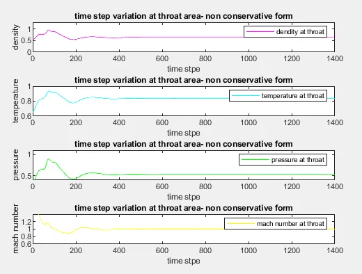
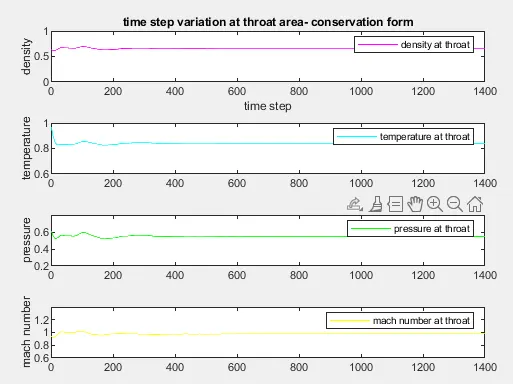
time step variation of primitive variable at throat area:

non- conservative:

conservative:

Observation:

From the above plots we can conclude that initial variation observed in non-conservative form for a certain period of time makes it consume higher amount of time to achieve stable solution when compared to conservative form.

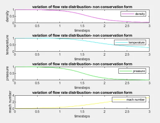
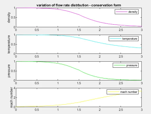
varation of flow rate distribution:

non-conservative form:

conservative form:

Observation:

Here by observing the above plots we could see that both the forms are in same phase giving the exact same solution for all the values.

mass flow rate at different time steps:

non-conservative form:

conservative form:

Observation:

Above plots shows that mass flow rate at different time steps along the distance oscillates initially, however the solution becomes stable after the 400^th Time step for both the forms attaining a constant value.

comprasion plot of normalized mass flow rate of both forms:

Observation:

Even though the final solution of both the forms are almost similar, the non-conservative form oscillates much when compared to conservative form. The latter also gives almost stable solution along the length. By this we can conclude that conservative form attains stability in lesser number of iteration with earliest time.

Conclusion:

Cumulating all the above result we can evidently conclude that conservative form converges slightly faster than non-conservative form offering stable solution along the simulation. Yet both the forms are dependable in calculating the solutions which is almost same.