Week 5 - Rayleigh Taylor Instability
Rayleigh Taylor Instability simulation
Aim:
- What are some practical CFD models that have been based on the mathematical analysis of Rayleigh Taylor waves? In your own words, explain how these mathematical models have been adapted for CFD calculations.
- Perform the Rayleigh Taylor instability simulation for 2 different mesh sizes with the base mesh being 0.5 mm. Compare the results by showing the animations( Attach them from your Google drive). Observe the differences in the animation and explain the effect of mesh size on simulation. Also, explain why a steady-state approach might not be suitable for these types of simulation.[ Choose Air and Water for this simulation]
- Run one more simulation with water and user-defined material (density = 400 kg/m3, viscosity = 0.001 kg/m-s) for refined mesh.
- Define the Atwood Number. Find out the Atwood number for both the cases and explain how the variation in Atwood number in the above two cases affects the behavior of the instability.
Introduction:
Rayleigh Taylor instability:
The Rayleigh Taylor instability, or RT instability (after Lord Raleigh and G.I Taylor), is an instability of an interface between two fluids of different densities which occurs when the lighter fluid is pushing the heavier fluid. Examples include supernova explosions in which expanding core gas is accelerated into shell gas.
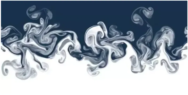
Water suspended atop oil is an everyday example RT instability, and it may be modeled by two completely plane – parallel layers of immiscible fluids, the more dense on top of the less dense one and both subject to the earth’s gravity. The equilibrium here is unstable to any perturbations or disturbances of the interface.
If a parcel of heavier fluid is displaced downward with an equal volume of lighter fluid displaced upwards, the potential energy of the configuration is lower than the initial state. Thus the disturbance will grow and lead to a further release of potential, as the more dense material moves down under the (effective) gravitational field, and the less dense material is further displaced upwards. This was the set-up as studied by Lord Rayleigh. The important insight by G.I. Taylor was his realization that this situation is equivalent to the situation when the fluids are accelerated, with the less dense fluid accelerating into the more dense fluid. This occurs deep underwater on the surface of an expanding bubble and in a nuclear explosion.
As the RT instability develops, the initial perturbations progress from a liner growth phase into a non-linear growth phase, eventually plumes flowing upwards (in the gravitational buoyancy sense) and spikes falling downwards. In the linear phase the fluid movement can be closely approximated by linear equation and the amplitude of perturbations is growing exponentially with time. In the non-linear phase, perturbation amplitude is too large for a linear approximation, and non-linear equation are required to between the fluids determines the structures of the subsequent non-linear RT instability flows (assuming other variable such as surface tension and viscosity are negligible here). The different in the fluid densities divided by their sum is defined as the Atwood number. For a close to 0, RT instability flows take the form of symmetric fingers of fluid. For A close to 1, the much lighter fluid below the heavier fluid takes the form of larger bubble- like plumes.
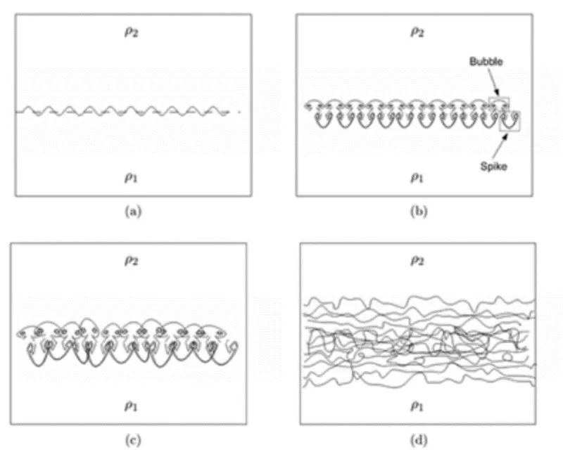
Practical CFD models that have been based on the mathematical analysis of Rayleigh Taylor waves.
Kelvin – Helmholtz instability:
It typically occurs when there is velocity shear in a single continuous fluid, or additionally where there is a velocity difference across the interface between two fluids. A common example is seen with wind blowing over water, the instability constant is able to manifest itself through waves on a water surface. The Kelvin – Helmholtz instability is not only restricted to a water surface as clouds, but is evident through other natural phenomena as the ocean.
The theory predicts the onset of instability and transition to turbulent flow with in fluids of different densities moving at various speeds. Helmholtz studied the dynamic of two fluids of different densities when a small disturbance, such as a wave, was introduced at the boundary connecting the fluids. Kelvin – Helmholtz instability can thus be characterized as unstable small scale motions occurring vertically and laterally. At times, the small scale instabilities can be limited through the prescience of a boundary. The boundaries are evident in the vertical direction through an upper and lower boundary.
Richtmyer – Meshkov instability (RMI):
The Richtmyer – Meshkov instability (RMI) occurs when two fluids of different density are impulsively accelerated. Normally this by the passage of a shock wave. The development of the instability begins with small amplitude perturbations which initially grow linearly with time. This is followed by a non-linear regime with bubbles appearing in the case of a light fluid penetrating a heavy fluid, and with spikes appearing in the case of a heavy fluid penetrating a light fluid. A chaotic regime eventually is reached and the two fluids mix.
Plateau – Rayleigh instability:
The Plateau – Rayleigh instability, often just called. The Rayleigh instability, explain why and how a falling stream of fluid breaks up into smaller packets with the same volume but less surfaces area. It is related to the Rayleigh and is part of a greater branch of fluid dynamics concerned with fluid thread breakup. This fluid instability is exploited in the design of a particular type of link jet technology where by a jet of liquid is perturbed into a steady stream of droplets.
Procedure:
Pre-processing:
Geometry:
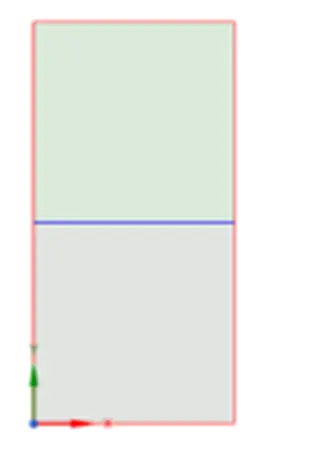
- A 2d rectangle sketch is drawn in space claim along XY axis using the sketch plane and using pull option is made into a surface.
- This surface is moved to a new component and named furthermore water surface is created in the similar way above the air surface.
- Using share topology from workbench the interacting edge is shared between the two surfaces.
Meshing:
Base mesh size: 0.5mm
The geometry is important from space claim and the mesh size is set to 0.5mm.
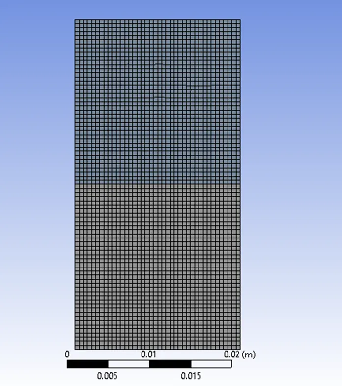
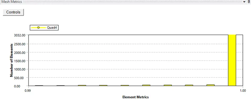
- No of nodes: 3321.
- No of elements: 3200.
Set-up:
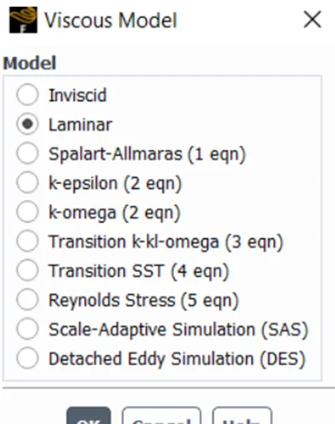
Laminar flows is selected and the transient state is selected and the gravity along the Y axis is given.
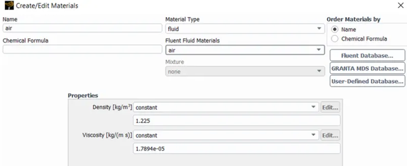
Air and water are selected from the fluent database.
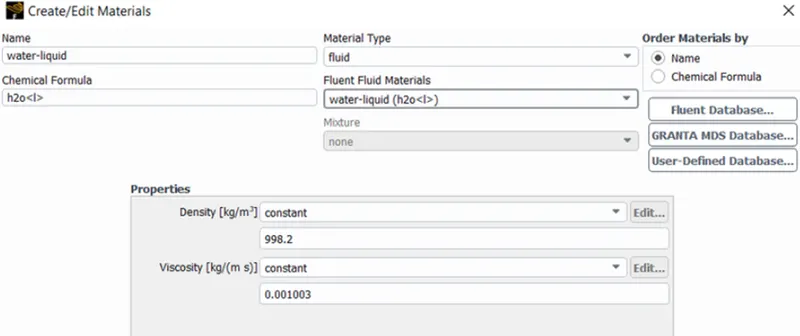
In the multiphase option the implicit method is selected and the phase are set according (water above and air below).
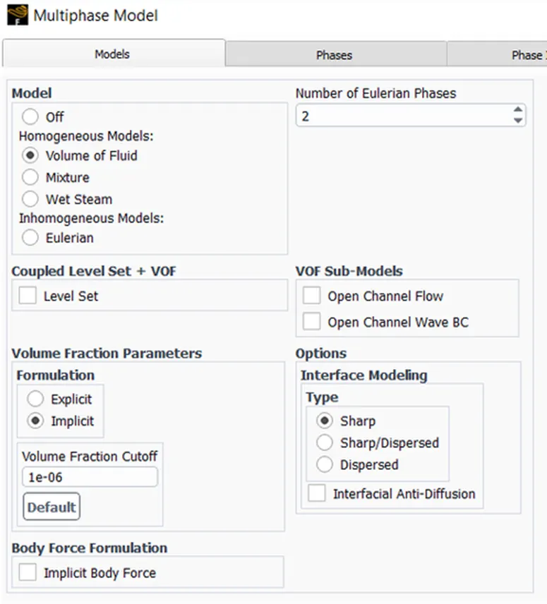
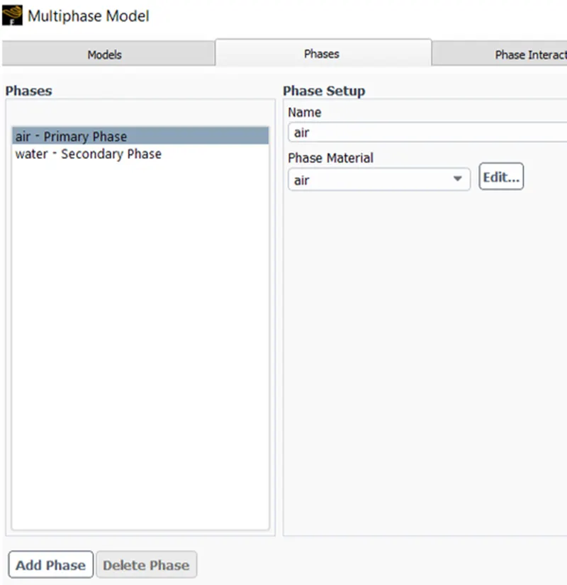
Then the set-up is initiated and after this, using the patch option is used to assign the identity value (alpha 1 = water; alpha 0 =air).
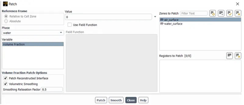
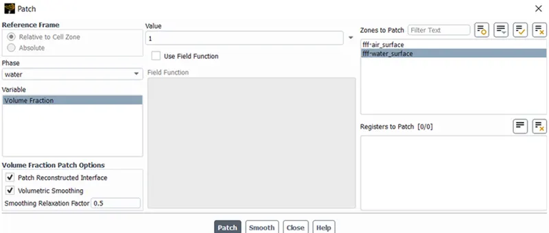
Time step size is set to 0.005 and the iterations are continued for 1500 time step.
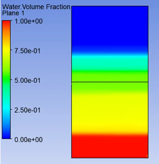
A contour plot is created for the phase – volume fraction – water and all the surfaces are selected and an animation is created for every time step.
Water volume fraction:
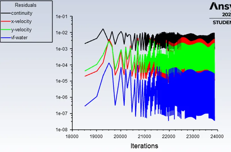
Residuals:
Animation:
Finer mesh size: 0.2mm:
The space claim geometry created above is used here as well but the mesh size has reduced to 0.2mm.
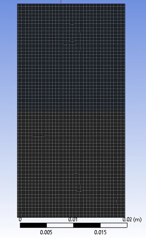
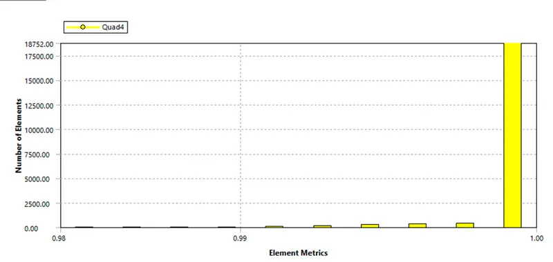
No of nodes: 20301.
No of elements: 20000.
Residuals:
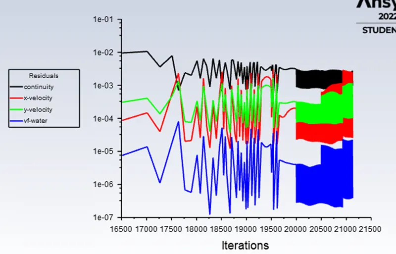
Animation:
User – defined:
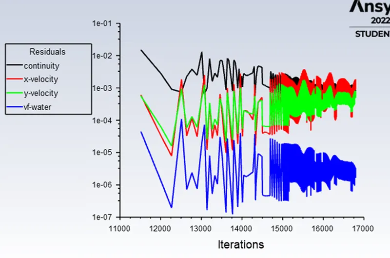
All the steps and values used in the refined mesh are used here as well but instead of air, a user defined elements with density 400 Kg/m3 and viscosity 0.001 Kg/m.s is used.
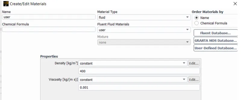
Residuals:
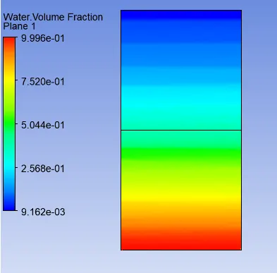
Water volume fraction:
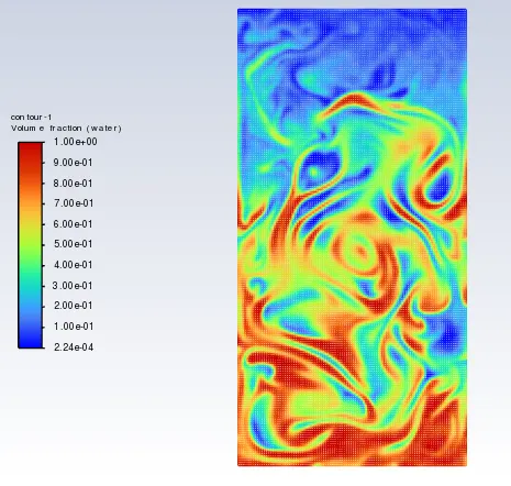
Animation:
Atwood number:
The Atwood number (A) is a dimensionless number in fluid dynamic used in the study of hydrodynamic instabilities in density stratified flows. It is a dimensionless density ratio defined as.
Where,
Rho 1 = density of heavier fluid.
Rho 2 = density of lighter fluid.
Case1:
Density of water = 998.2 Kg/m3
Density of air = 1.225 Kg/m3
Applying these values in the Atwood number formula.
Case2:
Density of water = 998.2 Kg/m3
Density of user defined substance = 400 Kg/m3
Applying these values in the Atwood number formula.
Observation:
Increasing the mesh size resulted in a finer simulation.
In the case of user defined element the immediate transition as seen in the air and water mixture in not seen.
Conclusion:
Thus the simulation and analysis of the Rayleigh Taylor instability between water and air has been done.