Week 5.1 - Mid term project - Solving the steady and unsteady 2D heat conduction problem
- Steady state analysis & Transient State Analysis
Solve the 2D heat conduction equation by using the point iterative techniques that were taught in the class. The Boundary conditions for the problem are as follows;
Top Boundary = 600 K
Bottom Boundary = 900 K
Left Boundary = 400 K
Right Boundary = 800 K
You will implement the following methods for solving implicit equations.
- Jacobi
- Gauss-seidel
- Successive over-relaxation
Your absolute error criteria is 1e-4
Introduction:
Explicit method:
When a direct computation is made for an unknown quality in terms in terms of know quality. This computation is a called explicit. This method requires stability criteria which when satisfied leads to stable solution. Because of the stability criteria small time has to be taken obtained stable solution. With decrease in time step the number of computation increases and hence the computational time required for the solution to converge is less and accuracy of solution is high.
Implicit method:
When a computation is made or dependent variable are define by set of equations and matrix is involved to find the unknown variable. This computation is called implicit method.
In order to solve for dependent variable iterative solvers are used.
Jacobi solver
Gauss seidal solver
Successive over relaxation solver
2D heat conduction equation:
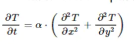
The time derivative term is hyperbolic in nature which can be discretized using forward differencing scheme and the special derivatives are elliptical in nature which can be discretized using central differencing scheme
Discretization of time derivative using forward scheme since the time derivative is varying in time direction which can be solved by marching method.
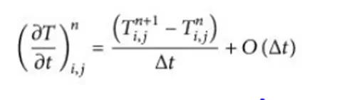
Discretization of special derivatives using central differencing scheme since the special derivatives are elliptical in nature, which uses information from neighboring points to obtain a solution.

From the PDE heat conduction equation:
 Where n is current time steps and n+1 is next time step.
Steady state 2D heat conduction equation:
Steady state is where the fluid properties does not change with respect to time.
From the 2D heat conduction equation since the system is in steady state time derivative is zero and diffusivity is constant.
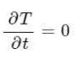
Hence we the equation for steady state as:-
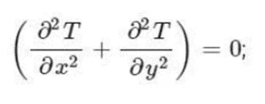
Discretization for steady state;
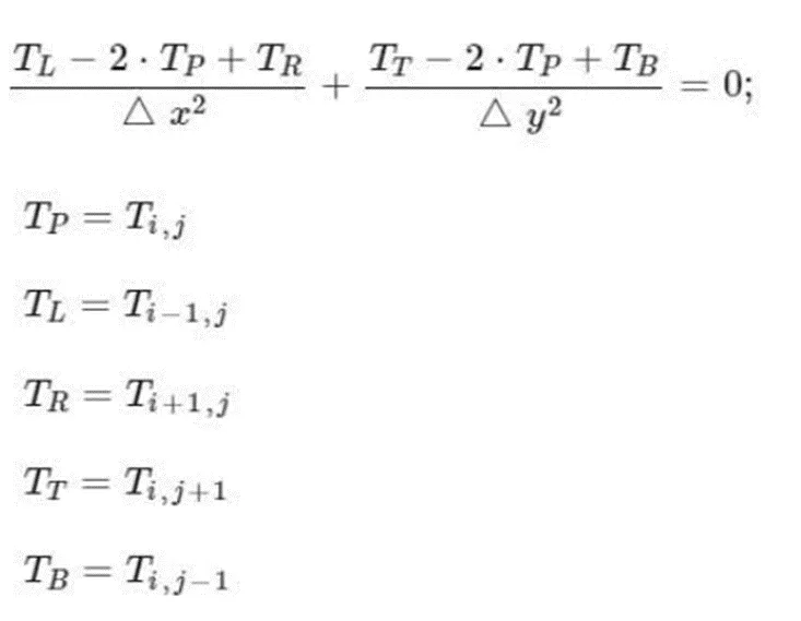
Solving for T(i, j), we get.
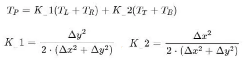
Formula for Jacobi iterative solver:

Formula for gauss seidal iterative solver:
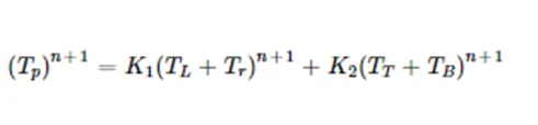
Formula for SOR iterative solver:

Transient state:
Unsteady state is where the fluid properties changes with respect to time.
The formula for 2D transient heat conduction equation is
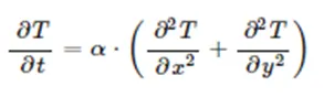
Discretization for unsteady state heat conduction equation
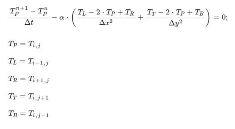 Solving 2D transient heat conduction equation explicitly we get.
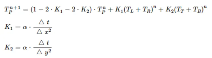
Stability criteria
K1 + k2 ≤ 0.5 stability criteria for 2D heat conduction equation when solving explicitly.
Solving 2D transient heat conduction equation implicitly we get.
Here n+1 is the next time step and n is the proceeding time step.
Formula for Jacobi iterative solver:
 Formula for gauss seidal iterative solver:

Formula for SOR iterative solver:

matlab main codes:
1. steady sates:
clear all
close all
clc
% inputs
nx=20; % number of grids in x direction
ny=nx; % number of grids in y direction
alpha= 0.3; % thermal diffucisity
omega=1.2; % sor initial value
tol=1e-4; % tolorence
error=9e9; % error value
T=5; % time limit
dt=1e-2; % time step
x=linspace(0,1,nx); % x axis mesh
y=linspace(0,1,ny); % y axis mesh
% grid spacing
dx= x(2)-x(1);
dy=y(2)-y(1);
[xx,yy]=meshgrid(x,y);
% matrix defromation
t= 300*ones(nx,ny); % initial temperatures gauss
t(end,:)=600; % top face
t(1,:)=900; % bottom face
t(:,1)=400; % left face
t(:,end)=800; % right face
k=(2*(dx^2+dy^2)/(dx^2*dy^2));
t_old=t;
t_p=t;
%% soving method
method='which method?';
solver=input(method); % '1'steady state jacobi methot
% '2'steady state gauss sedial method
% '3'steady state SOR method
% jacobi method
if solver ==1
iter_1=1;
tic;
% convergence loop
while (error>tol)
for i=2:(nx-1) % loop equation
for j=2:(ny-1) % loop summation
TL=t_old(i-1,j);
TR=t_old(i+1,j);
TT=t_old(i,j+1);
TB=t_old(i,j-1);
H=(TL+TR)/dx^2;
V=(TT+TB)/dy^2;
t(i,j)=(H+V)/k;
end
end
time=toc;
error=max(max(abs(t_old-t)));
t_old=t;
iter_1=iter_1+1;
[x,y]=contourf(xx,yy,t);
colormap(jet)
colorbar
clabel(x,y)
pause(0.03)
title_text1 = sprintf('steady state heat counduction using jacobi= %d',iter_1);
title_text2 = sprintf('simulation time +%f s',time);
title_text3 = sprintf('finial error=%f',error);
title({title_text1;title_text2;title_text3})
end
end
%% gauss sedial method
if solver==2
iter_2=1;
tic;
% convergence loop
while (error>tol)
for i=2:(nx-1) % loop equation
for j=2:(ny-1) % loop summation
TL=t(i-1,j);
TR=t(i+1,j);
TT=t(i,j+1);
TB=t(i,j-1);
H=(TL+TR)/dx^2;
V=(TT+TB)/dy^2;
t(i,j)=(H+V)/k;
end
end
time2=toc;
error=max(max(abs(t_old-t)));
t_old=t;
iter_2=iter_2+1;
time=toc;
[x,y]= contourf(xx,yy,t)
colormap(jet)
colorbar
clabel(x,y)
pause(0.03)
title_text1 = sprintf('steady state heat counduction using gauss sedial = %d',iter_2);
title_text2 = sprintf('simulation time +%f s',time);
title_text3 = sprintf('finial error=%f',error);
title({title_text1;title_text2;title_text3})
end
end
%% SOR
if solver==3
iter_3 = 1
tc;
% convergence loop
while (error>tol)
for i=2:(nx-1) % loop equation
for j=2:(ny-1) % loop summation
TL= t(i-1,j);
TR= t_old(i+1,j);
TT= t_old(i,j+1);
TB= t(i,j-1);
H= (TL+TR)/dx^2;
V= (TT+TB)/dy^2;
tgs(i,j)= (H+V)/k;
t(i,j)= t_old(i,j)*(1-omega)+omega*tgs(i,j);
end
end
time3=toc;
error=max(max(abs(t_old-t)));
t_old=t;
iter_3=iter_3+1
time=toc;
[x,y]=contourf(xx,yy,t);
colormap(jet);
colorbar;
clabel(x,y);
pause(0.03);
title_text1 = sprintf('steady state heat counduction using SOR = %d',iter_3);
title_text2 = sprintf('simulation time +%f s',time);
title_text3 = sprintf('finial error=%f',error);
title({title_text1;title_text2;title_text3});
end
end
As from stated on the figure, the number of iteration required to converge the solution is more in Jacobi iteration schemes followed by gauss sedial iteration and SOR scheme. Which obviously means the computational time required for a computer program to run the iteration is more in Jacobi followed by gauss sedial and SOR schemes
For explicit scheme, we cannot use the same time steps and length of mesh domain, as it yield to high CFL number, which leads to unstable solution converging. For the convenient I have taken the time steps and length domain for both x and y axis mentioned in the code section.
2. transient implicit:
clear all
close all
clc
%% inputs
nx= 20; % number of grids in x direction
ny= nx; % number of grids in y direction
alpha= 1.4; % thermal diffucisity
omega= 1.2; % initial value of sor
tol= 1e-4; % tolorence
error=9e9; % error value
T= 5; % time limits
dt=1e-2; % time steps
x=linspace(0,1,nx); % x axis mesh
y=linspace(0,1,ny); % y axis mesh
%grid spacing
dx=x(2)-x(1);
dy=y(2)-y(1);
[xx,yy]= meshgrid(x,y);
% matrix deformation
t= 300*ones(nx,ny); % initial temperatures gauss
t(end,:)=600; % top face
t(1,:)=900; % bottom face
t(:,1)=400; % left face
t(:,end)=800; % right face
k1= alpha*dt/dx^2;
k2= alpha*dt/dy^2;
k= 1+(2*k1)+(2*k2);
t_old= t;
t_p= t;
%% solving method
method= 'which method? ';
solver= input(method); % '1' jacobi
% '2' gauss sedial
% '3' SOR
%% jacobi
if solver== 1;
iter_1= 1;
tic;
% convergence loop
while (error>tol);
for i= 2:(nx-1) % loop equation
for j= 2:(ny-1) % loop summation
TL= t_old(i-1,j);
TR= t_old(i+1,j);
TT= t_old(i,j+1);
TB= t_old(i,j-1);
H= TL+TR;
V= TT+TB;
t(i,j)= ((t_p(i,j)+H*k1+V*k2)/k);
end
end
time= toc;
error= max(max(abs(t_old-t)));
t_old=t;
iter_1= iter_1+1;
[x,y]= contourf(xx,yy,t);
colormap(jet);
colorbar
clabel(x,y);
pause(0.03);
title_text1= sprintf('transient state heat counduction using implicity jacobi = %d',iter_1)
title_text2= sprintf('sumulation time +% f s', time)
title_text3= sprintf('final error = %f',error)
title({title_text1;title_text2;title_text3})
end
end
%% gauss sedial
if solver== 2;
iter_2=1;
tic;
% loop convergence
while (error>tol);
for i= 2:(nx-1); % loop equation
for j= 2:(ny-1); % loop summuation
TL = t(i-1,j);
TR = t_old(i+1,j);
TT = t(i,j+1);
TB = t_old(i,j-1);
H = TL+TR;
V = TT+TB;
t(i,j) = ((t_p(i,j)+H*k1+V*k2)/k);
end
end
time1=toc;
error= max(max(abs(t_old-t)));
t_old=t;
iter_2= iter_2+1
time=toc;
[x,y]= contourf(xx,yy,t);
colormap(jet);
colorbar;
clabel(x,y);
pause(0.03);
title_text1= sprintf('transient state heat counduction using implicity gauss sedial = %d',iter_2)
title_text2= sprintf('sumulation time +% f s', time)
title_text3= sprintf('final error = %f',error)
title({title_text1;title_text2;title_text3})
end
end
%% SOR
if solver ==3;
iter_3 = 1
tic;
% loop convergence
while (error>tol)
for i = 2:(nx-1) % loop equation
for j = 2:(ny-1) % loop summation
TL = t(i-1,j);
TR = t_old(i+1,j);
TT = t(i,j+1);
TB = t_old(i,j-1);
H= TL+TR;
V= TT+TB;
tgs(i,j)= ((t_p(i,j)+H*k1+V*k2)/k);
t(i,j)= (1-omega)*t_old(i,j)+omega*tgs(i,j);
end
end
time3=toc;
error= max(max(abs(t_old-t)));
t_old=t;
iter_3= iter_3+1;
time=toc;
[x,y]= contourf(xx,yy,t);
colormap(jet);
colorbar;
clabel(x,y);
pause(0.03);
title_text1= sprintf('transient state heat counduction using implicity SOR = %d',iter_3)
title_text2= sprintf('sumulation time +% f s', time)
title_text3= sprintf('final error = %f',error)
title({title_text1;title_text2;title_text3})
end
end
3. transient explicit:
clear all
close all
clc
%% inputs
nx= 10; % number of grids in x direction
ny= nx; % number of grids in y direction
alpha= 0.3; % thermal diffucisity
omega= 1.2; % initial value of sor
tol= 1e-4; % tolorence
error=9e9; % error value
T= 5; % time limits
dt=1e-2; % time steps
nt=T/dt;
x=linspace(0,1,nx); % x axis mesh
y=linspace(0,1,ny); % y axis mesh
%grid spacing
dx=x(2)-x(1);
dy=y(2)-y(1);
[xx,yy]= meshgrid(x,y);
% matrix deformation
t= 300*ones(nx,ny); % initial temperatures gauss
t(end,:)=600; % top face
t(1,:)=900; % bottom face
t(:,1)=400; % left face
t(:,end)=800; % right face
k1= alpha*dt/dx^2;
k2= alpha*dt/dy^2;
k= 1-(2*k1)-(2*k2);
t_old =t;
t_p=t;
%% solving method
method= 'which method? ';
solver= input(method); % '1' jacobi
% '2' gauss sedial
% '3' SOR
%% jacobi
if solver== 1;
iter_1= 1;
nt=T/dt;
tic;
for m=1:nt
while (error>tol);
for i= 2:(nx-1) % loop equation
for j= 2:(ny-1) % loop summation
TL= t_old(i-1,j);
TR= t_old(i+1,j);
TT= t_old(i,j+1);
TB= t_old(i,j-1);
H= TL+TR;
V= TT+TB;
t(i,j)= t_p(i,j)*k+H*k1+V*k2;
end
end
error=max(max(abs(t-t_old)));
t_old=t;
iter_1=iter_1+1
end
t_p=t;
end
time1=toc;
[x,y]= contourf(xx,yy,t);
colormap(jet);
colorbar;
clabel(x,y);
pause(0.03);
title_text1= sprintf('transient state heat counduction using explicity jacobi = %d',iter_1)
title_text2= sprintf('sumulation time +% f s', time1)
title_text3= sprintf('final error = %f',error)
title({title_text1;title_text2;title_text3})
end
%% gauss sedial
if solver ==2
iter_2= 1
nt=T/dt
tic;
for m= 1:nt
while (error>tol)
for i= 2: (nx-1)
for j= 2: (ny-1)
TL = t(i-1,j);
TR = t_old(i+1,j);
TT = t(i,j+1);
TB = t_old(i,j-1);
H= TL+TR;
V= TT+TB;
t(i,j) = t_p(i,j)*k+H*k1+V*k2;
end
end
error=max(max(abs(t-t_old)));
t_old=t;
iter_2=iter_2+1
end
t_p=t;
end
time3=toc;
[x,y]= contourf(xx,yy,t);
colormap(jet);
colorbar;
clabel(x,y);
pause(0.03);
title_text1= sprintf('transient state heat counduction using explicity gauss sedial = %d',iter_2)
title_text2= sprintf('sumulation time +% f s', time3)
title_text3= sprintf('final error = %f',error)
title({title_text1;title_text2;title_text3})
end
%% SOR
if solver ==3
iter_3= 1
nt=T/dt
tic;
for m= 1:nt
while (error>tol)
for i= 2: (nx-1)
for j= 2: (ny-1)
TL = t(i-1,j);
TR = t_old(i+1,j);
TT = t(i,j+1);
TB = t_old(i,j-1);
H= TL+TR;
V= TT+TB;
tgs(i,j) = t_p(i,j)*k+H*k1+V*k2;
t(i,j) = (1-omega)*(t_old(i,j))+omega*tgs(i,j);
end
end
error=max(max(abs(t-t_old)));
t_old=t;
iter_3=iter_3+1
end
t_p=t;
end
time3=toc;
[x,y]= contourf(xx,yy,t);
colormap(jet);
colorbar;
clabel(x,y);
pause(0.03);
title_text1= sprintf('transient state heat counduction using explicity SOR = %d',iter_3)
title_text2= sprintf('sumulation time +% f s', time3)
title_text3= sprintf('final error = %f',error)
title({title_text1;title_text2;title_text3})
end
Results:
Comparing with the different iteration approaches and states, we can conclude the following things
- The computational time and iteration required are SOR<GAUSS<JACOBI for both steady and unsteady states.
- Steady states are less complicated to analyses because time marching properties change has been avoided, on the other transient states approach deals with more sophisticated and complicated unknown and considering of time marching phenomena changes such as diffusion rates
- Between explicit and implicit result, the latter one does not depend greatly on courant number for its stability and convergence, on the other hand in the explicit approach information from a given cell or mesh element must propagate to its immediate neighbors, hence the low CFL number needs to be considered.