Week 4.1: Project - Steady state simulation of flow over a throttle body

Steady state simulation of flow over a throttle body

Aim:

The aim of this challenge is to simulate the flow over a throttle body inside an elbow.

Objective:

• Simulation of flow over a throttle body.
• Post processing of the results for flow variables.

Throttle body:

In an internal combustion engine, the throttle is a means of controlling an engine's power by regulating the amount of fuel or air entering the engine. In a motor vehicle the control used by the driver to regulate power is sometimes called the throttle, accelerator, or gas pedal. For a gasoline engine, the throttle most commonly regulates the amount of air and fuel allowed to enter the engine. Recently. for a gasoline direct injection engine, the throttle regulates the amount of air allowed to enter the engine. The throttle of a diesel, when present, regulates the air flow into the engine.

Historically, the throttle pedal or lever acts via a direct mechanical linkage. The butterfly valve of the throttle is operated by means of an arm piece, loaded by a spring. This arm is usually directly linked to the accelerator cable, and operates in accordance with the driver, who hits it. The further the pedal is pushed, the wider the throttle valve opens.

Modern engines of both types (gas and diesel) are commonly drive-by-wire systems where sensors monitor the driver controls and in response a computerized system controls the flow of fuel and air. This means that the operator does not have direct control over the flow of fuel and air; the Engine Control Unit (ECU) can achieve better control in order to reduce emissions, maximize performance and adjust the engine idle to make a cold engine warm up faster or to account for eventual additional engine loads such as running air conditioning compressors in order to avoid engine stalls.

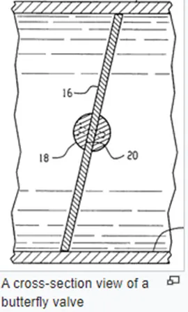
The throttle on a gasoline engine is typically a butterfly valve. In a fuel-injected engine, the throttle valve is placed on the entrance of the intake manifold, or housed in the throttle body. In a carbureted engine, it is found in the carburetor. When a throttle is wide open, the intake manifold is usually at ambient atmospheric pressure. When the throttle is partially closed, a manifold vacuum develops as the intake drops below ambient pressure.

The power output of a diesel engine is controlled by regulating the quantity of fuel that is injected into the cylinder. Because diesel engines do not need to control air volumes, they usually lack a butterfly valve in the intake tract. An exception to this generalization is newer diesel engines meeting stricter emissions standards, where such a valve is used to generate intake manifold vacuum, thereby allowing the introduction of exhaust gas (see EGR) to lower combustion temperatures and thereby minimize NOx production.

In a reciprocating engine aircraft, the throttle control is usually a hand-operated lever or knob. It controls the engine power output, which may or may not reflect in a change of RPM, depending on the propeller installation (fixed-pitch or constant speed).

Some modern internal combustion engines (such as some BMW engines) do not use a traditional throttle, instead relying on their variable intake valve timing system to regulate the airflow into the cylinders, although the end result is the same, albeit with less pumping losses.

Steady state simulation of throttle body:

Geometry:

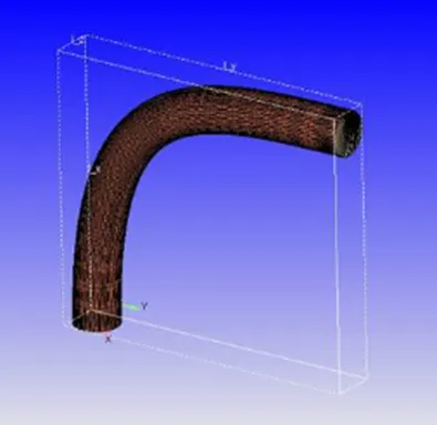
Elbow joint contains the throttle body over which we are interested to see the flow over the body.

Mesh:

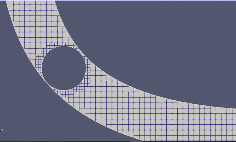
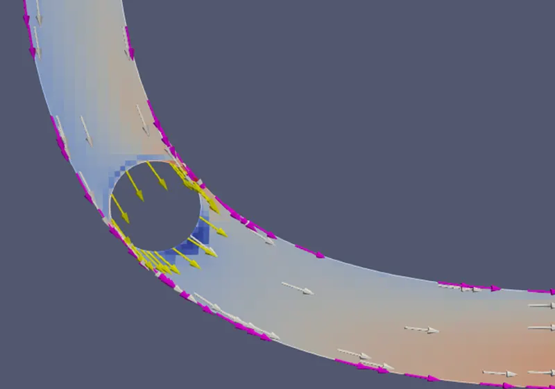
Figure shows the mesh structure developed by the cut cell Cartesian method. Base size of 0.002m base grid was formed as we can see near the holes, fixed embedding was employed to create a fine mesh around the body to study the flow parameters. Then we used the scale of 3 and added 2 layers of embedding to get this fine mesh.

Pre-processing:

Case set-up:

• Time based

Materials:

• Predefined mixtures – air (gas simulation)

Simulation parameters:

• Solver – pressure-based steady solver.
• Mode – full hydrodynamic.
• Start time – 0 cycles.
• End time – 1500 cycles.
• Initial time – 1e-9.
• Minimum time step – 1e-9.
• Maximum time step – 1 sec.

Regions and initialization:

• Add region (air).
• Pressure – 101325 pa.
• Species – air (O2 = 0.23, N2 = 0.77)

Boundary conditions:

Inlet boundary:

• Inflow boundary.
• Pressure = 1.5e⁵.
• Mixture = air.
• Temperature = 300k.

Outlet boundary:

• Outlet flow boundary.
• Pressure = 1e⁵.
• Mixture = air.
• Temperature = 300k.

Throttle:

• Wall boundary.
• Wall motion – stationary.
• Surface movement – fixed.
• Temperature boundary condition = law of wall 300k.
• Turbulent kinetic energy – zero normal gradient.
• Turbulent dissipation – wall motion.

Elbow wall:

• Wall boundary.
• Wall motion – stationary.
• Surface movement – fixed.
• Temperature boundary condition = law of wall 300k.
• Turbulent kinetic energy – zero normal gradient.
• Turbulent dissipation – wall motion.

Base grid:

• Mesh in dx, dy, dz = 0.002.

Fixed embedding:

Fixed embedding is used to refine the mesh around the desired regions. In this case the regions of interest are the inner walls of the channels. Therefore, the fixed embedding is applied with a scale of 3 and 2 embedded layers.

Output files:

Time interval to write 3D output data files – 1000.0 cycles.

Time means that after every 1000 cycles, 3D output data files will be written and saved.

Results:

Mass flow rate:

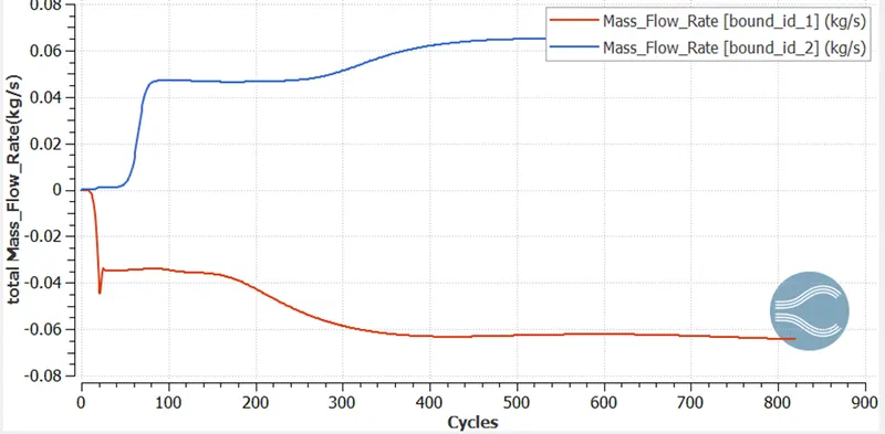
For a steady state simulation, it is most impotent to check if convergence has attained. To do so, it is a good idea to analyze mass flow rate plots for inlet and outlet section. Shows the plot for mass flow rate at the inlet and outlet section respectively.

We can see that the convergence for both the inlet and outlet section occurs at approx. 0.065 kg/s mass flow rate after approx. 400 cycles. The negative sign at the inlet indicates that the flow is into the system and the positive side at the outlet flows out of the system.

Total cell count:

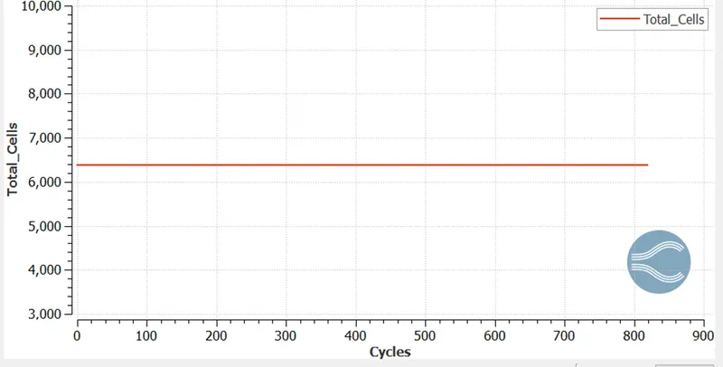
The geometry has been divided into around 820 cells which have been distributed evenly between the 4 processes. The graph for the total number of cells vs. No. of cycles plot.

Velocity contour:

Velocity plot:

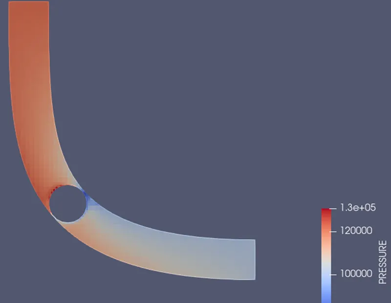
Pressure plot:

Pressure contour:

Conclusion:

• The simulation of flow over a throttle plate was run.
• Flow variables were analyzed using para view and converge line plot modules.
• The fundamental laws of fluid flow are conserved.