Week 6: Conjugate Heat Transfer Simulation

Conjugate Heat Transfer Simulation

Objective:

To simulate the flow through the solid pipe conjugate heat transfer and understand super cycling.

• Baseline configuration
• Setup a flow simulation through a pipe
• Inlet Reynolds number should be 7,000

HINT : Use the below formula to calculate velocity for corresponding value of REYNOLD NUMBER and give DIRICHLET BC for velocity at inlet and specify the value for velocity calculated at INLET BC using below formula ,

Re = (rho*V*D)/(Dynamic viscosity)

• Turbulence modelling - K-Epsilon
• Super cycling parameters - same as in the video
• Additional 3D outputs
• Add Y+ to your post.in file
• Grid dependence test
• Start with an initial base grid
• Run grid dependence test on 3 grids and show that the outlet temperature converges to a particular value
• Effect of supercycle stage interval
• Set supercyle stage interval to 0.01,0.02 and 0.03
• For these three values, how does the total simulation time compare against the baseline configuration

Boundary layer:

Now that we understand the importance of the boundary layer, let us look at its structure in detail. In the boundary layer, the velocity profile changes rapidly and can be broken up into three regions: viscous sublayer, log layer and outer layer, as shown in Figure 1 below.

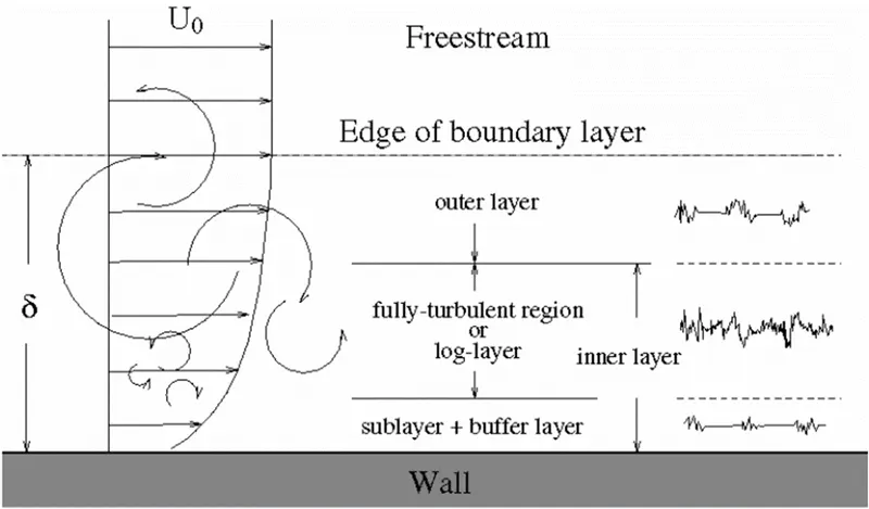
Figure 1 – Schematic of the velocity boundary layer

Resolving the boundary layer close to the wall provides an accurate representation of its profile, leading to accurate predictions of wall shear stress, surface pressure, the effect of adverse pressure gradients and forces.

There are large pressure gradients that must be resolved to accurately predict downforce and drag.

How does CFD resolve the boundary layer:

By using a log-scale and empirical equations to non-dimensionalise the velocity (u⁺) and the distance from the wall (y⁺), the velocity profile of the boundary layers takes on a predictable form, Figure 2. There are two other equations, as shown below by the red line in, shown via blue lines that have been derived capturing the profile of the viscous sublayer and the log-region.

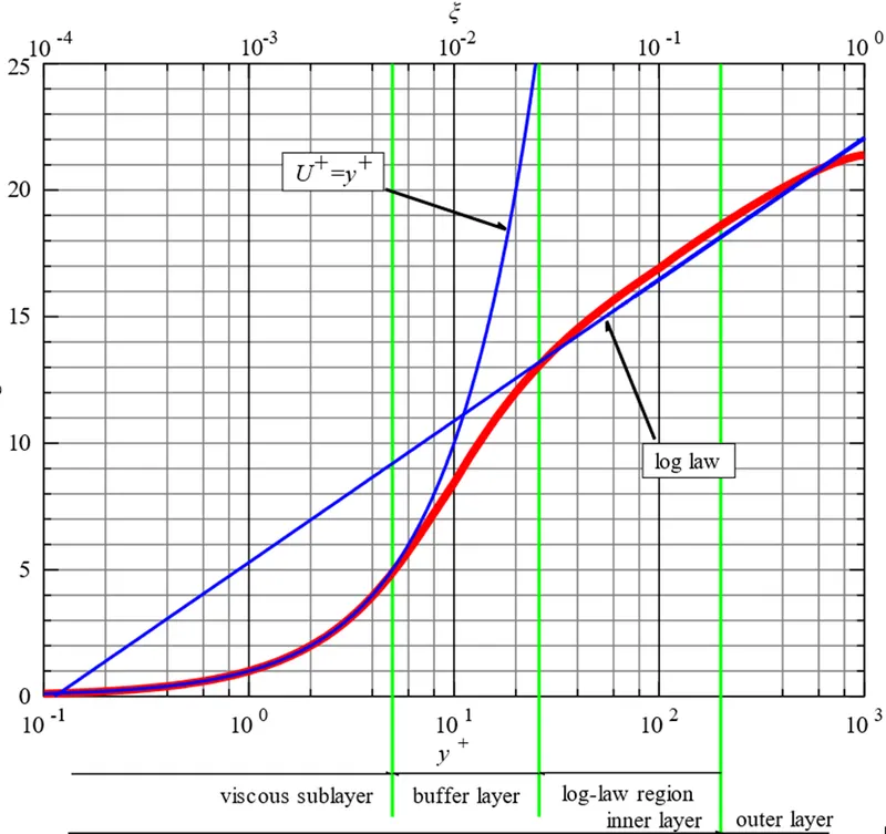
Figure 2 – Non-dimensional velocity versus distance from the wall

In CFD software the boundary layer is modelled by extruding the surface mesh elements at the wall. The surface mesh can be made up of different element types, but for the purposes of this discussion, we will consider triangular surface elements which are extruded into prism cells. The boundary layer resolution depends on the first cell height and the number of prism layers. The solver calculates a value, y⁺, which is computed from the first cell height, local flow speed and fluid properties. For the same fluid and flow conditions, we can say that reducing the first prism height by a factor of 2 will reduce y⁺ by a factor of 2. Obtaining an initial value for y⁺ and then adjusting the prism heights in the meshing tool or via adaption is a common practice in CFD when tuning the mesh for best results.

Different turbulence models are used to capture the boundary layer in different ways. The k-ω SST model has been widely researched, tested and is accepted as a good choice for many industrial problems, and has the robustness to resolve the viscous sublayer or the log layer. If the first cell height is in the viscous layer, it will resolve the boundary layer by evaluating the velocity at each cell. If the first cell is in the log layer, the software will make an empirical assumption about the viscous sublayer, referred to as using a wall function.

A careful selection of how you would like to model the boundary layer is essential.

When resolving the viscous sublayer, a value for y⁺~1 is required, which will require significantly more mesh elements and effort, Figure 3, left-hand image. This will lead to higher meshing and solution times and the requirement for more computer system resources. If you determine, that is not important to resolve the viscous sublayer, i.e. to use a wall function, a value for y⁺ > 30 is valid; this will result in less meshing effort and computational time, Figure 3, right-hand image. Note, however, that using wall functions can result in modelling errors, the significance of which will vary depending on flow conditions.

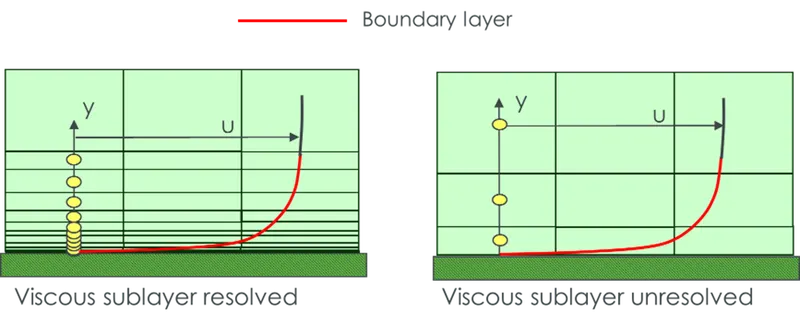
Figure 3 – Left – Near wall mesh when resolving the viscous sublayer, Right – Near wall mesh when using wall functions

It is recommended to either resolve the viscous sublayer by creating a mesh with y⁺~1 or to use the wall function approach by having the first element in the log region (y⁺ >30) and avoid having a y⁺ between those values.

Super cycling concept:

Super cycling is a technique which is used in converge studio in the case of conjugate heat transfer problem with a solid and liquid region. Main problem is that both solvers cannot run at the same speed since solving in fluid domains is much faster owing to the time scale difference for heat transfer in liquids as compared to the solids. This causes problem during the solution given that the solid side solver would not have reached a steady state/ converge in the time the liquid solver does. This is where the concept of super cycling is based.

The basic idea of super cycling is that the solver for the fluid domain is paused until the solver for the solid domain converges. The following steps are involved in performing the super cycling.

• Solve the fluid and the solid together with the transient solver. Store the instantaneous heat transfer coefficient and temperature on the interface during process.
• Freeze the fluid solver. Time-average the heat transfer coefficient and temperature and applies them as boundary conditions at the interface
• Solves the solid temperature until it reaches steady-state.
• Update the solid temperature field and unfreezes the fluid solver.
• Repeats until the solid temperature converges.

Calculate velocity at inlet based on Reynolds numbers:

Given:

Re.No = 7000;

Inner diameter (fluid region diameters) = 0.03D.

At 300K, properties of air at 1atm pressure.

Density = 1.161 kg/m³.

Dynamic viscosity = 0.00001846 kg/ms.

Velocity calculation based on Reynolds numbers.

v = R_e. μ / ρ D; = (7000).(0.00001846) / (1.161).(0.03) = 3.71m/s.

Skin friction drag co-efficient = C_f = 0.058 R_e^{-1/3 (}for external flows)

C_{f =} (0.058) (7000 ^-1/3) = 0.0098720736.

Wall shear stress = τ = ½ (C_f) (ρ) (U²).

= ½ (0.0098720736)*(1.161)*(3.71²).

τ = 0.0788784611 N/M².

Frictional velocity = u_t =

= = 0.2606532261.

Assume the desired Y⁺ = 32.

The first cell center to boundary distance = Y⁺ *v/u_t

= 32* (0.000015859 / 0.2606532261) = 0.0019469853 m.

Geometry dimensions:

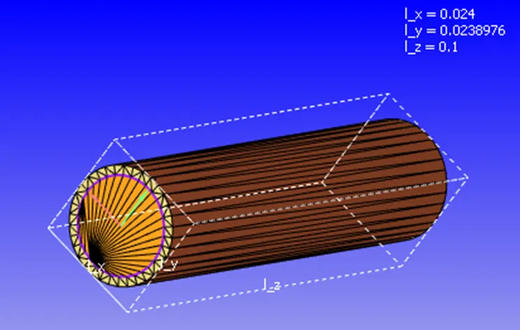
• The non-manifold problems occurs due to the presence of three surface of a triangular element in contact with each other which are not recommended in ordinary simulation but are unavoidable in CHT analysis. This error will automatically disappear after the case setup procedure as converge identifies this simulation to be CHT analysis.

Case-setup:

• In order to begin the case-setup, click on the case-setup and click begin case-setup and click time based.
• Then click on materials and select air to be predefined mixtures. Also enable the solid simulation and species.
• Then open the gas simulation and global transport parameters and retain the default setting. Then open the species tab, in the query available list choose the aluminum as a solid species. Then go to gas and in the query available list, choose N2 and O2 as a gas species.
• then click on the run parameter under the simulation parameter and choose the transient solver under the solver tab and then choose the full hydrodynamic under the simulation mode and then choose the compressible under the gas flow solver.
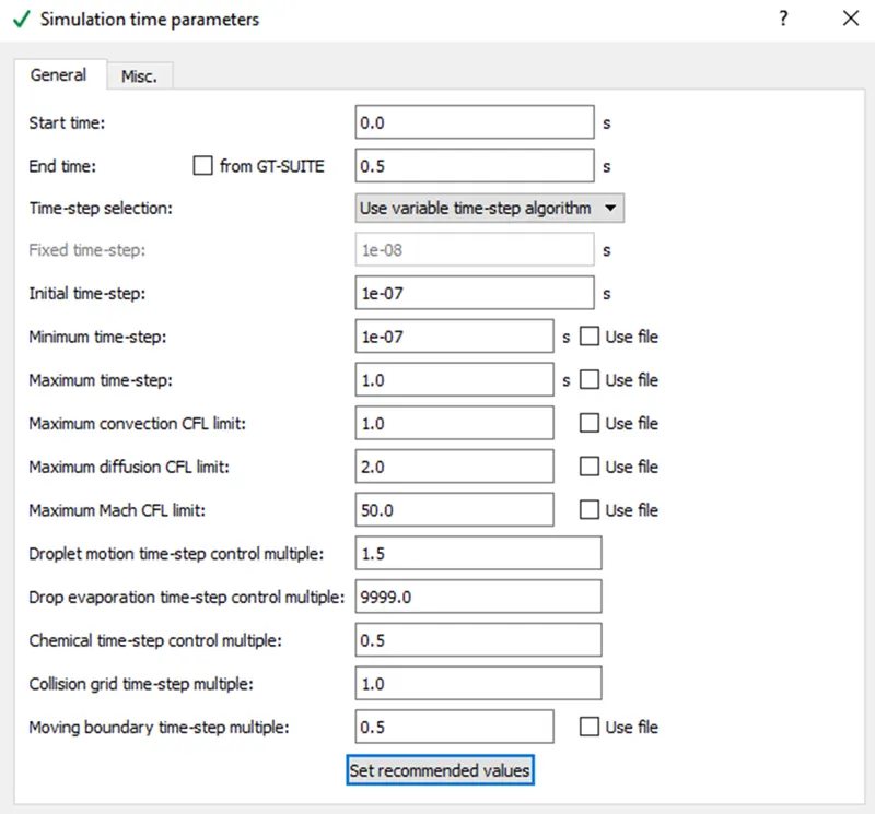
• In the simulation time parameter do the following changes.
• 
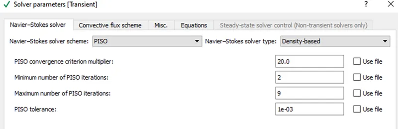
• In the solver time parameter, we only choose the pressure based solver and retain the remaining setting

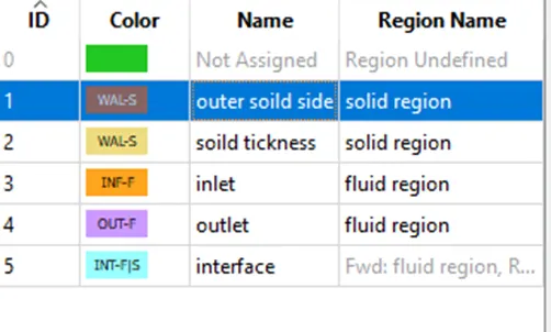
• Add the boundaries by clicking create multiple boundaries to create all boundaries at a once and name them like outer solid side, solid thickness, inlet, outlet, interface, by selecting the respective triangles.

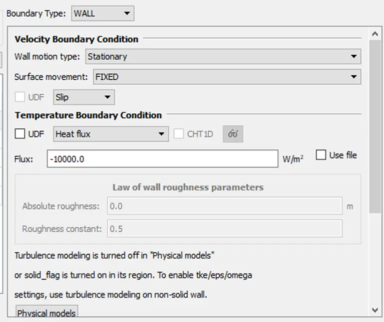
• In the outer solid side, we select the boundary type as a wall. And we are choosing the -10000 as a heat flux in the temperature boundary condition. And also select the region as a solid region.

• In the solid thickness, we are choosing the wall type boundary condition the velocity boundary condition as a slip. And temperature boundary condition as a zero normal gradient. And also select the region as a solid region.
• 
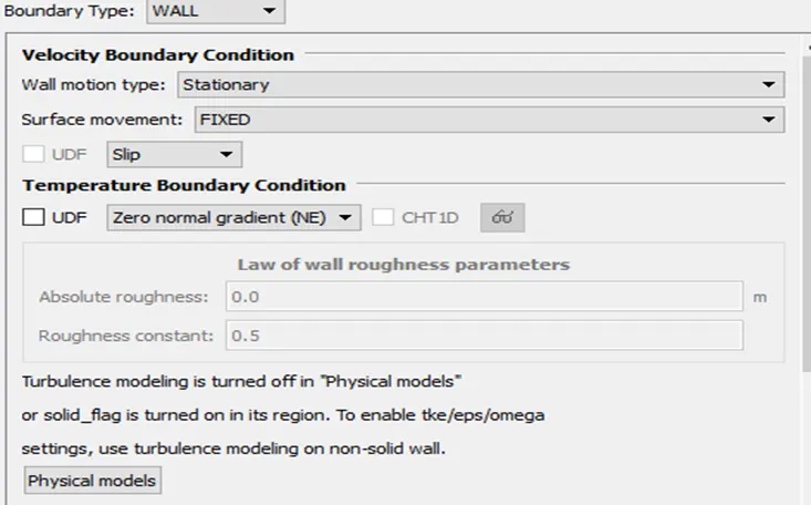
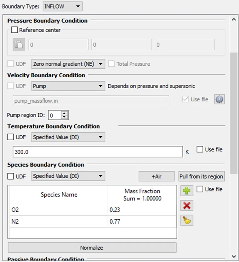
• We are choosing the boundary type as an inflow. And also select the region as a fluid region. Choose the zero normal gradient in the pressure boundary condition. in the velocity boundary condition choose 3.71 m/s in the z-positive direction. And we are selecting the 300K in the temperature boundary condition. And select the air as a species.

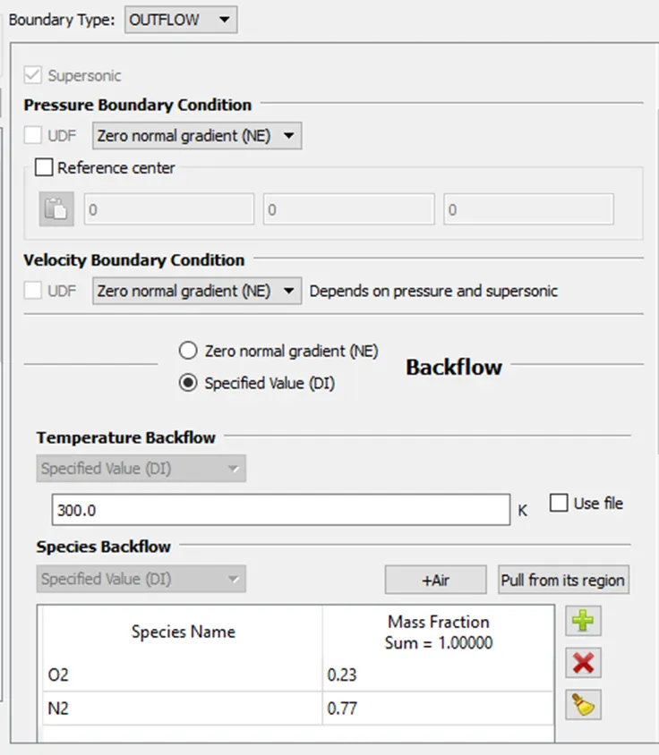
• Choose outflow as the boundary type and select the region as the fluid region. Pressure boundary are specified as a 101325pa. And we are choosing the velocity boundary condition as a zero normal gradient choose 300K temperature as a backflow boundary condition. And for species backflow, we are choosing the air.

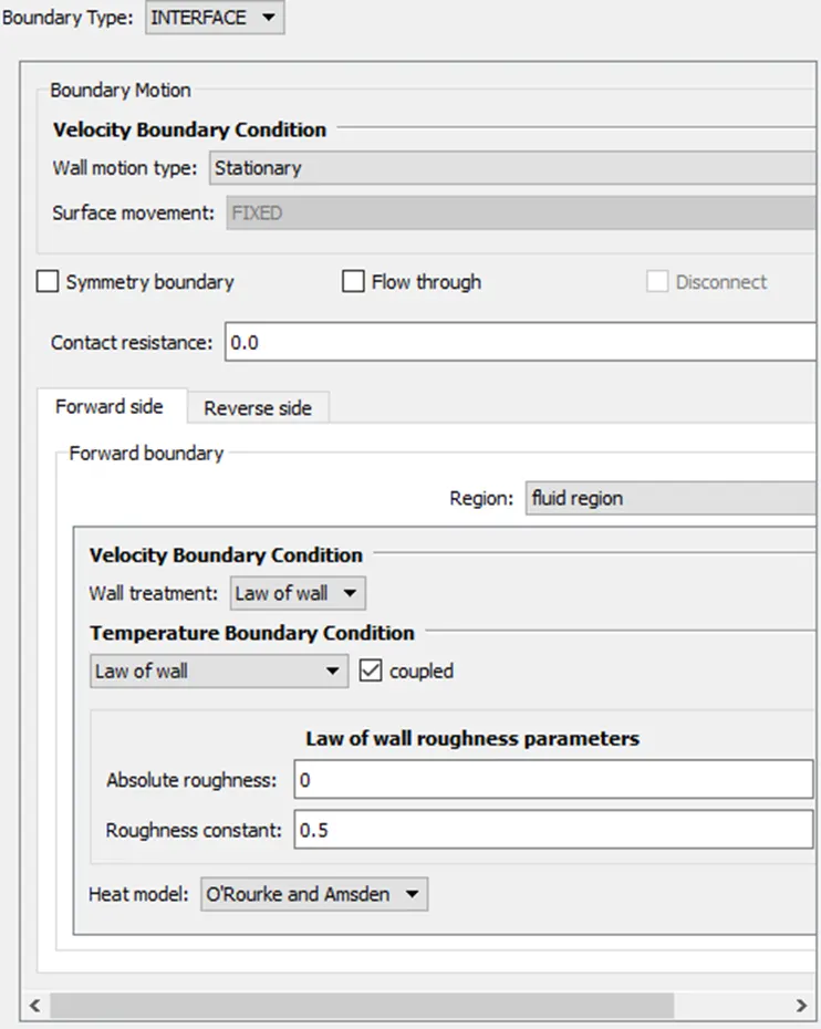
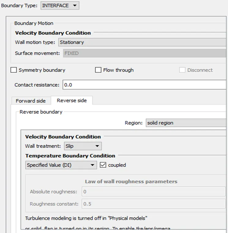
• In interface, it has forward and reverse direction.
• If you have hide the inlet boundary, we can see that normal are pointing towards the fluids domain that direction is called the forward direction for an interface boundary.
• If the normal pointing towards the solid, then the forward direction indicates the solid region.
• Internally we are going to say that we have two boundaries forward and revers boundary. Internally when converge runs, it’s going to create the copy of the interface boundary, one belonging to the fluid side and other belonging to the other side.
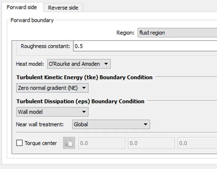
• So far the forward boundary that is toward the fluid region. And for the fluid region the boundary need the law of wall boundary condition.
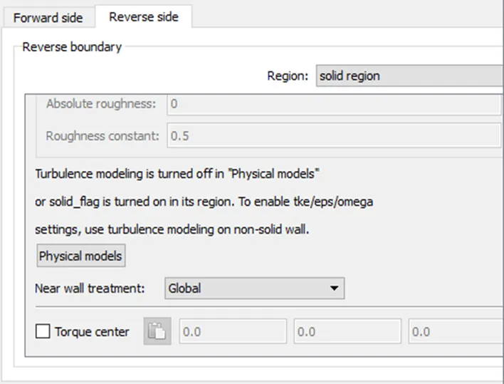
• And for the reverse region pointing toward the solid region.

Forward side boundary condition

Reverse boundary condition

• In regions and initialization, click add as region-0 and region-1.

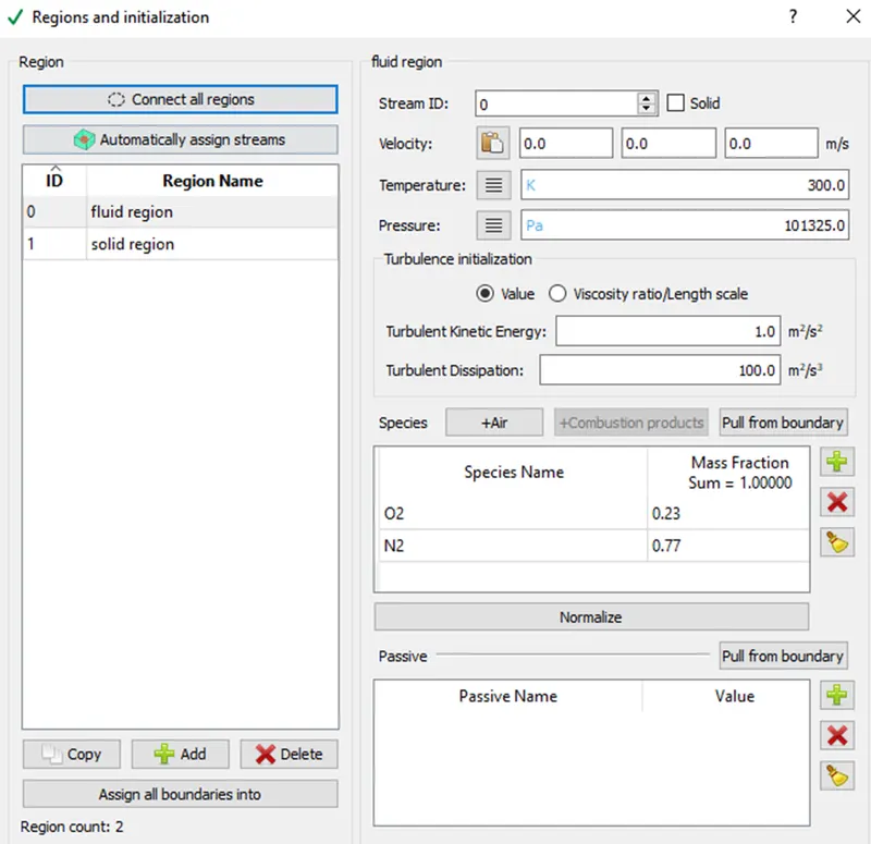
• In the fluid region set the stream-id as 0 and velocity condition as (0, 0, 0). Temperature initial condition as 300K and pressure condition as 101325 pa.

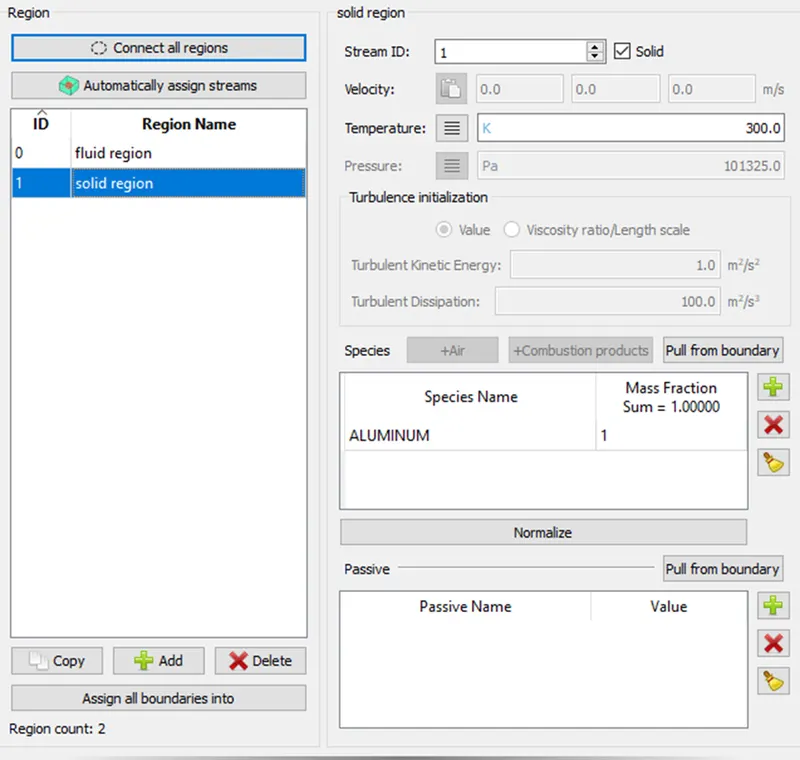
• In the solid region set the stream-id as 1. Set the temperature boundary condition as 300K. Specify the boundary condition as aluminum with a mass fraction of 1.00.
• Then go to physical modelling and enable the turbulence and super cycling modelling.

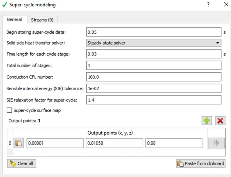
• The first option is to set the initial time at which the super-cycle begins storing data. This can be set from 0 to any value less than or equal to the total simulation time.
• The solvers used for the solid region can be a steady or transient solver that is independent of the solver set in the run parameters.
• The time length of each cycle determines the intervals at which the fluid domain is paused and the solid domain solved for. This interval is taken into account after the initial paused of the fluid solver at 1.
• The CFL number, SIE tolerance and relaxation factors are solver parameters that are given for the purpose of accuracy and speed of the solver.
• An output point must be defined in the solid region to let the solver know at which the temperature data must be calculated. This point must be given in the solid domain as the solver runs for the solid domain and once this value converges, the fluid domain solver is continued.
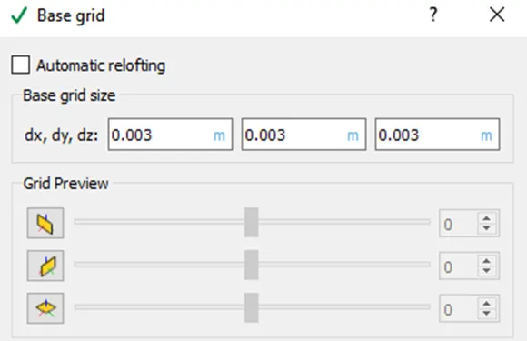
• We are running the simulation using three base grid which is 0.001, 0.002 and 0.003.

• Now we are select the post variables. Then go to post variables selecting → combustion / turbulence → and enabled the Y⁺. And retain the remaining setting.
• Then open the output files and do the following setting.

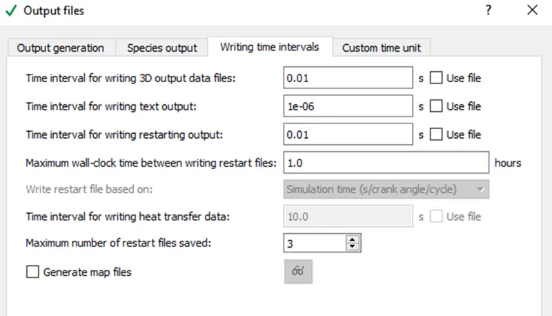
• At the end all the inputs files have to be exported.

Results:

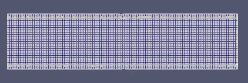
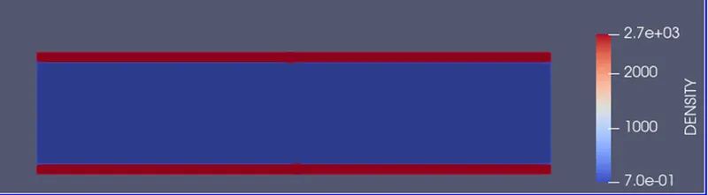
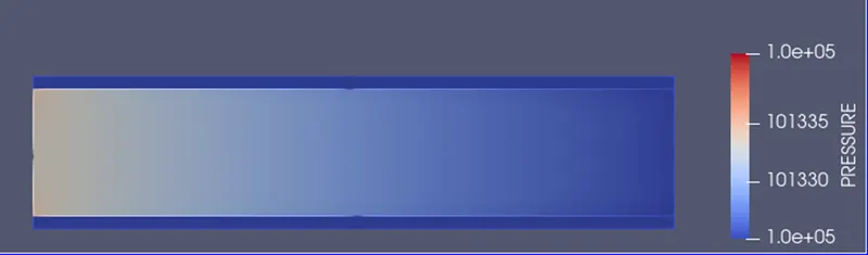
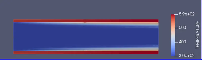
Case 1: super cycle stage interval 0.01, mesh grid 0.001

Mesh:

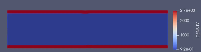
Density:

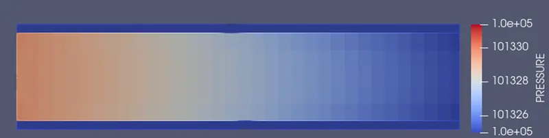
Pressure:

https://youtu.be/wY3n0CoXWik

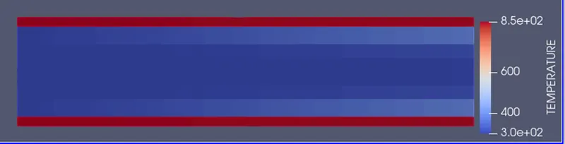
Temperature:

https://youtu.be/BGooqKw-fxs

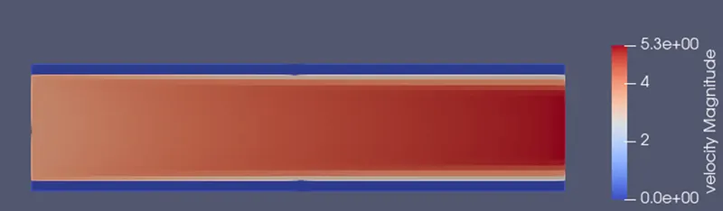
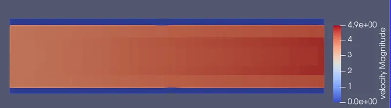
Velocity:

https://youtu.be/IH0N91ZVtqU

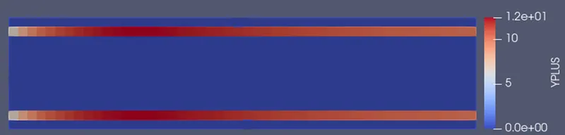
Y plus:

https://youtu.be/-ECyKaJ4LVg

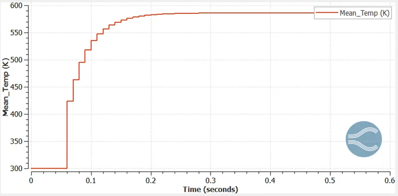
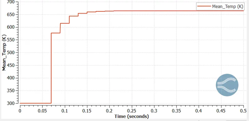
Mean temperature:

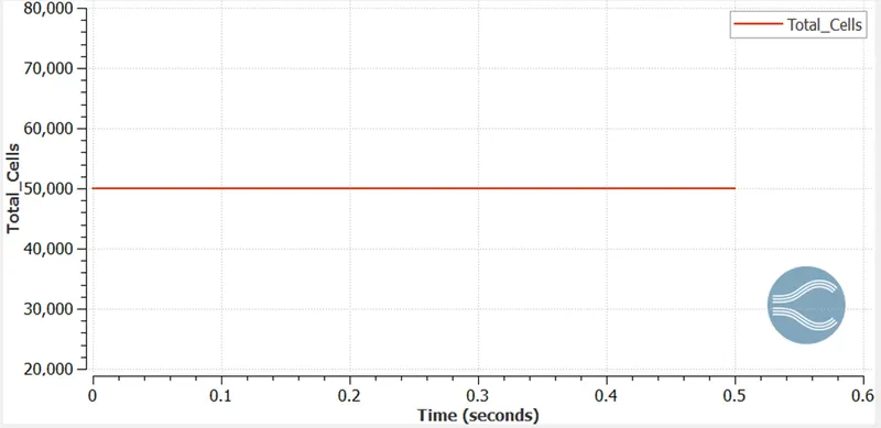
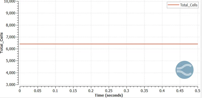
Total cell count:

Case 2: super cycle stage interval 0.02, mesh grid 0.002

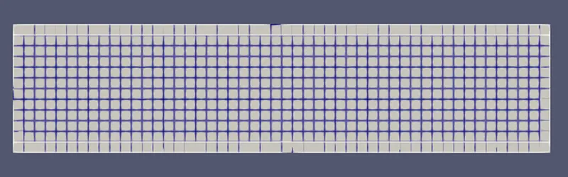
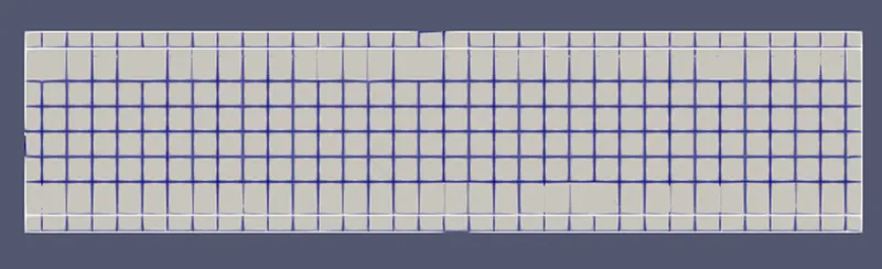
Mesh:

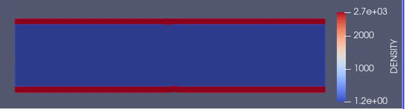
Density:

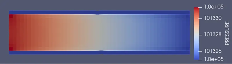
Pressure:

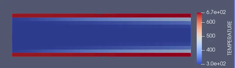
Temperature:

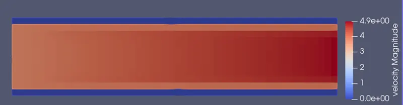
Velocity:

Y plus:

Mean temperature:

Total cell count:

Case 3: super cycle stage interval 0.03, mesh grid 0.003.

Mesh:

Density:

Pressure:

Temperature:

Velocity:

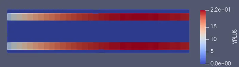
Y plus:

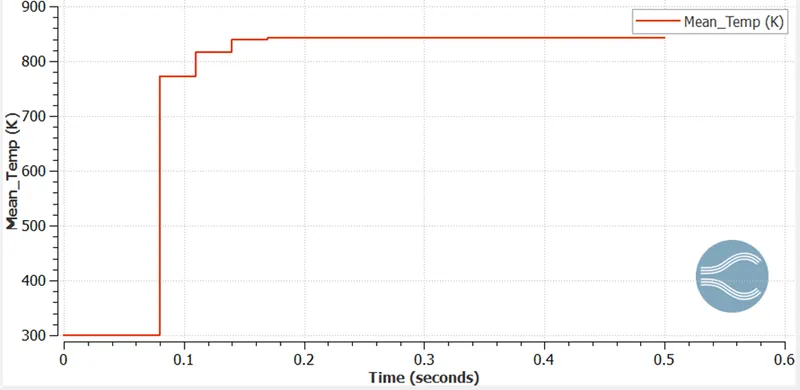
Mean temperature:

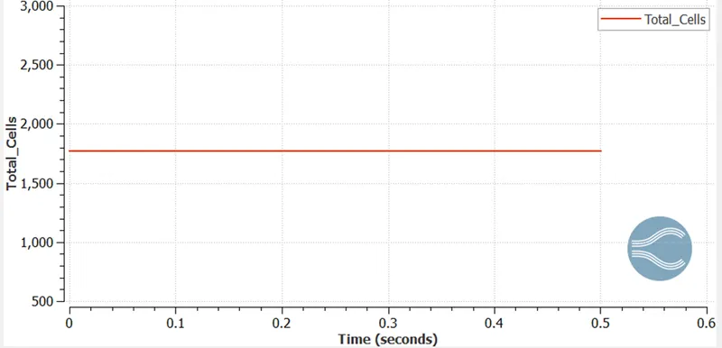
Total cell count:

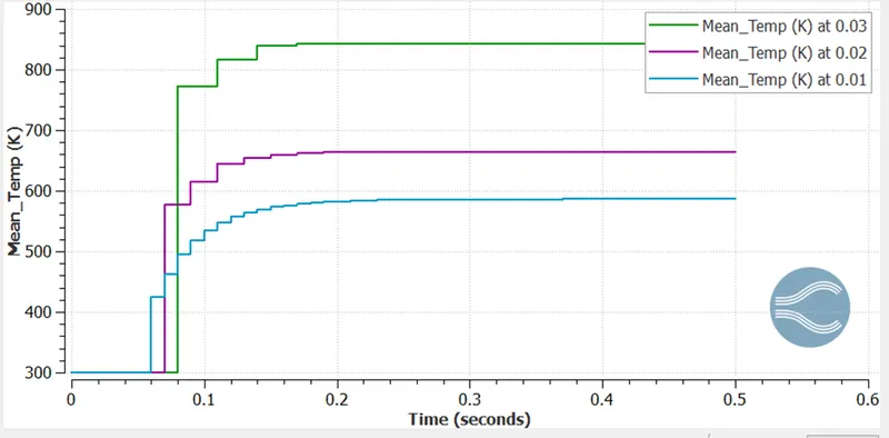
Total mean temperature:

Conclusion:

• Super-cycling helps to reduce overall simulation time.
• By knowing the Y+ value the first cell height of the mesh near the boundary or interface of wall can be calculated. As the mesh size decreases, the Y+ decreases, cell size also decreases, and cell counts increase.
• The temperature of fluid is maximum at the wall due to friction and heat transfer from the solid surface.
• The velocity of fluid is maximum at the center of the cylinder, whereas it is minimum near the wall due to viscosity.
• As the super-cycling time intervals is less, the temperature plot converge faster.
• As the mesh become finer, the accuracy of the temperature results increases.