Week 1 : Exploring the GUI of GT-POWER

Explore the GUI SUITE and list down modules available with brief description.

GT - Suite is the CAE simulation tool with capabilities and libraries aimed at a wide range of application and industries. It offer engineering functionalities ranging from fast concept design to detailed system or sub system/component analysis, design optimization and root couse investigation.

Industries used GT – Suite

• On highway vehicle.
• Off-highway vehicle.
• Marine and rail.
• Industrial machinery.
• Power generation.

Multi physics platform

The foundation of GT–Suite is a versatile multi physics platform for constructing models of general system based on many underlying fundamental libraries.

• Flow library (any fluid, gas or liquid or mixture).
• Acoustics library (both linear and nonlinear).
• Thermal library (all types of heat transfer).
• Mechanical library (kinematics, multi – body dynamics, frequency domain).
• Electric and electromagnetic library (circuit, electromechanical devices).
• Chemistry library (chemical kinetics)
• Controls library (signal processing)
• Built in 3D CFD and 3D FE (thermal and structural)

Modern software and unique capabilities

• Fusion of 1D and 3D simulation in one tool.
• Imports solid models from CAD to create 1D and 3D models.
• Performs embedded 3D (CFD) and 3D FE thermal/structural modeling with all boundary conditions provided by the simulated surrounding complete system.

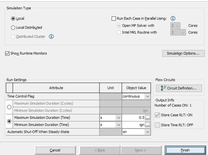
Time control flag:

In the below image we can see the time control flag option.

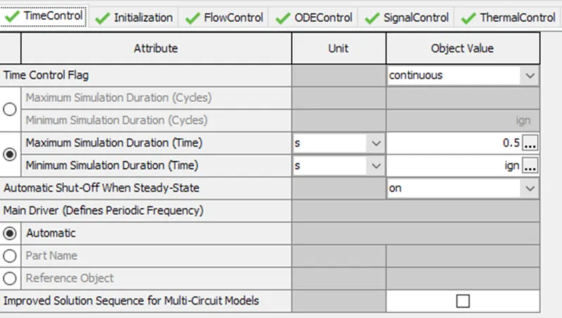
Defines the global simulation type with regard to time. One of the following options.

Periodic:

Periodic indicates that the model contains at least one circuit which contains a periodic event (i.e. engine cylinder ‘cycle’) and therefore requires tracking of results with respect to angle over each cycle. Any model that includes an ‘engine Crank Train’, ’Crank analysis’, or ‘Engine Crank Shaft’ part should use the periodic option. Note that the simulation duration for a periodic simulation can be specified in cycles or in time, whichever is most convenient.

Continuous:

Continuous indicates that the simulation includes no periodic event, and therefore has no need to track results with respect to a cyclic angle. This is the typical setting for models that contain only quasi – steady fluid circuits such as coolant or under hood air. This simulation duration for a continuous simulation is typically specified in time.

Time step and solution control:

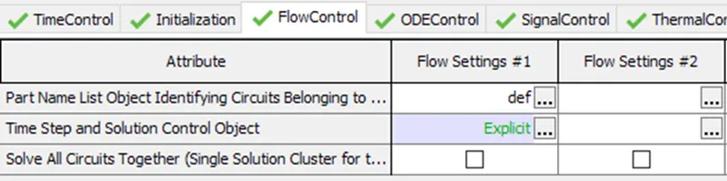
• Name of the ‘flow control Explicit’, ‘Flow control implicit’, ‘flow control QS’, reference object that can be used to define the numerical parameters for the explicit, implicit or quasi-steady flow solver, respectively.
• If there are no flow circuits in the model, starting in V2016 build 2 this attribute may be set to ‘ign’ or left blank (which is a rate exception to the normal requirement in GT-Suite that all cells must be filled).

Integrator/solver type:

• Integrator/solver type used in the time-marching of all ODEs including mechanical, electrical and magnetic libraries. For recommendations based on the application, please see the color-code table immediately following this text.

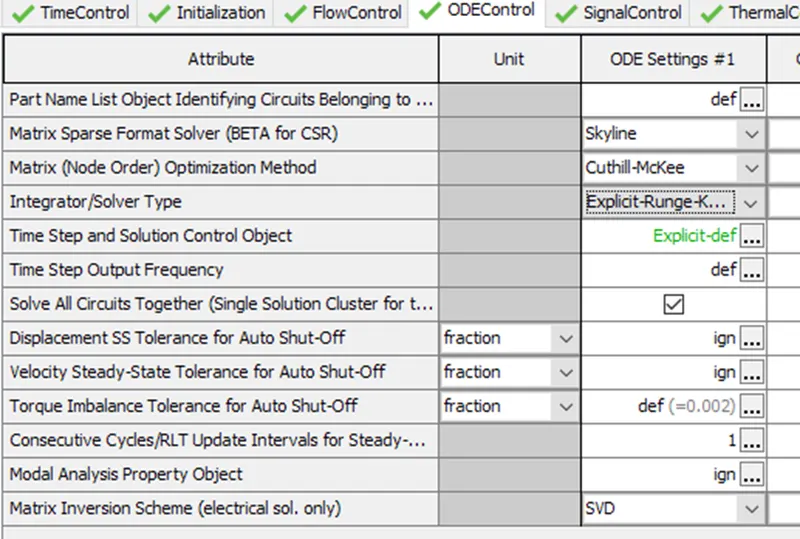
Explicit-Adams-PECE:

Explicit Adams-Bashforth-Moulton predictor-corrector integration scheme with variable order accuracy. This integrator is recommended for large non-stiff problems, problems with a high maximum time step which have different scales and real time applications. It requires a tuning process in order to optimize its functionality, please contact Email: [email protected] for more details.

Explicit Runge-Kutta:

Integration scheme that is 5 th order accurate. This integrator is recommended for non-stiff problem

Implicit – trapezoidal:

Implicit Trapezoidal integration scheme that is 2 nd order accurate. This integrator is recommended for moderately stiff problems.

Implicit-H.H.T:

Implicit Hilber-Hughes-Taylor integration scheme that is 2 nd order accurate. This integrator is recommended for moderately stiff problems.

Implicit – Radau 2:

Implicit 2-stage Radau integration scheme that is 3 rd order accurate. This integrator is recommended for stiff problems.

Implicit – Radau 3:

Implicit 3-stage Radau integration scheme that is 5 th order accurate. This integrator is recommended for stiff problems.

Implicit-S.D.C.3:

Implicit 3-stage Spectral Deferred Correction (S.D.C.) integration scheme that is 5th order accurate. This integrator is recommended for very stiff problems.

Intercooler Tutorial:

• Open the GT suite and click on Files and then select Tutorials then select Engine Performance and then 6cylDITurbo and then select the intercooler final.gtm.
• Thus the intercooler set up will pop up on the screen.

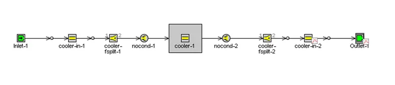
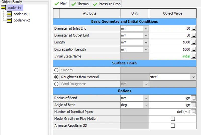
Define inlet and outlet diameter = 50mm.

Length = 1000mm.

Material = steel.

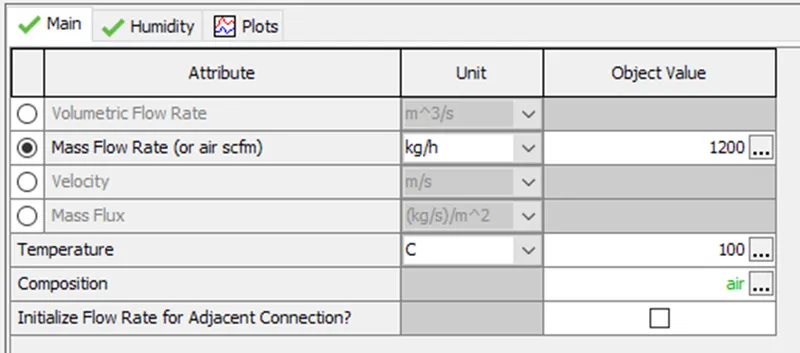
Mass flow rate in intercooler = 1200 Kg/h.

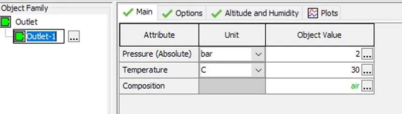
Outlet parameter is 2bar at 30deg C.

Run setup:

Run the case after input all parameters and open result with GT post processor.

Results:

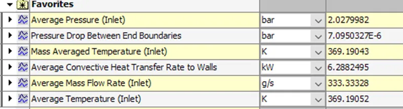
Average heat transfer to walls = 6.2882 KW.

Pressure drop between End boundaries = 7.09e-6 bar.

Conclusion:

This is project, the GUI of the GT-Suite was explored and the different setting were student. In the end, the tutorial case for the intercooler available in the GT-Suite library was simulation and results were extracted.