Week 5: Prandtl Meyer Shock problem
To Simulate The Prandtl- Meyer Shock Flow
Aim:
To Simulate the prandtl- meyer shock flow in converge CFD.
Shock (fluid dynamics):
Shock is formed due to coalescence of various small pressure pulses. Sound waves are pressure waves and it is at the speed of the sound wave the disturbances are communicated in the medium. When an object is moving in a flow field the object sends out disturbances which propagate at the speed of sound and adjusts the remaining flow field accordingly. However, if the object itself happens to travel at speed greater than sound, then the disturbances created by the object would not have traveled and communicated to the rest of the flow field and this results in an abrupt change of property, which is termed as shock in gas dynamics terminology.
Shocks are characterized by discontinuous changes in flow properties such as velocity, pressure, temperature, etc. Typically, shock thickness is of a few mean free paths (of the order of 10−8 m). Shocks are irreversible occurrences in supersonic flows (i.e. the entropy increases).
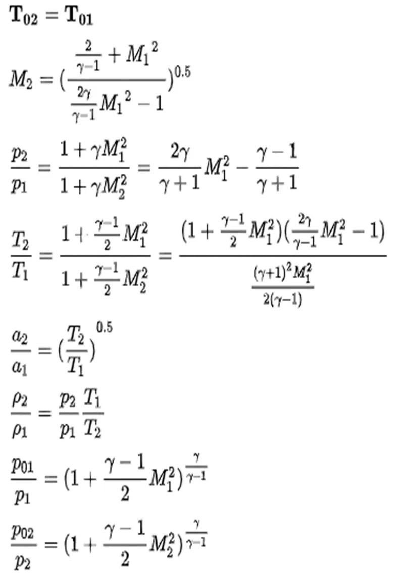
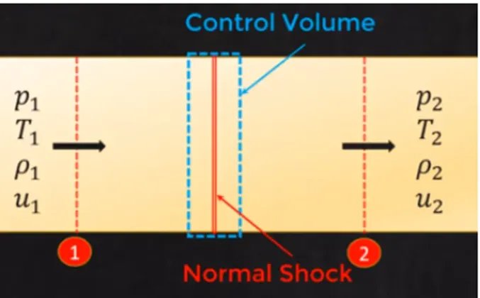
Normal shock formulas:
Prandtl-Meyer function:
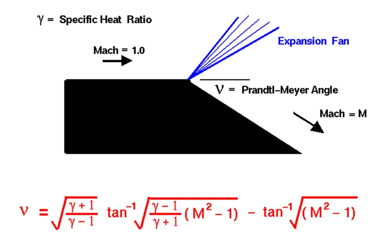
As an object moves through a gas, the gas molecules are deflected around the object. If the speed of the object is much less than the speed of sound of the gas, the density of the gas remains constant and the flow of gas can be described by conserving momentum and energy. As the speed of the objects increases towards the speed of sound, we must consider compressibility effects on the gas. The density of the gas varies locally as the gas is compressed by the object. When an object moves faster than the speed of sound, and there is an abrupt decrease in the flow area, shock waves are generated. If the flow area increases, however, a different flow phenomenon is observed. If the increase is abrupt, we encounter a centered expansion fan.
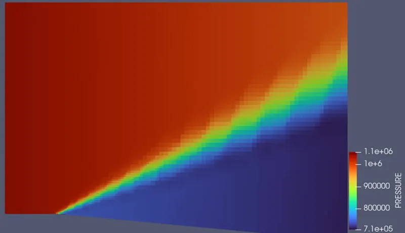
There are some marked differences between shock waves and expansion fans. Across a shock wave, the Mach number decreases, the static pressure increases, and there is a loss of total pressure because the process is irreversible. Through an expansion fan, the Mach number increases, the static pressure decreases and the total pressure remains constant. Expansion fans are isentropic.
The calculation of the expansion fan involves the use of the Prandtl-Meyer function. This function is derived from conservation of mass, momentum, and energy for very small (differential) deflections. The Prandtl-Meyer function is denoted by the Greek letter nu on the slide and is a function of the Mach number M and the ratio of specific heats gam of the gas.
nu={sqrt[(gam+1)/(gam-1)]}*atan{sqrt[(gam-1)*(M^2-1)/(gam+1)]}-atan{sqrt[M^2 -1]}
where atan is the trigonometric inverse tangent function. It is also written as shown on the slide tan^-1. The meaning of atan can be explained by these two equations:
atan(a) = b
tan(b) = a
As mentioned above, the Mach number of a supersonic flow increases through an expansion fan. The amount of the increase depends on the incoming Mach number and the angle of the expansion. The physical interpretation of the Prandtl-Meyer function is that it is the angle through which you must expand a sonic (M=1) flow to obtain a given Mach number. The value of the Prandtl-Meyer function is therefore called the Prandtl-Meyer angle.
Waves in compressible flow:
Gas flow over a body creates a disturbance that propagates through the fluid domain and interacts with other parts of the body. These disturbances are called waves and their motion is referred to as wave motion.
Two features of compressible waves are shock waves and expansion waves.
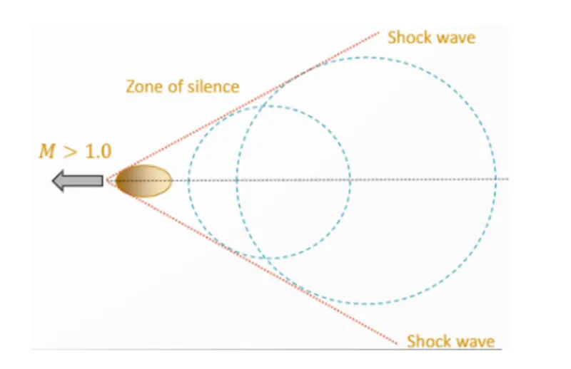
A shock wave is a fluid flow disturbance propagating through the gas faster than the local speed of sound. As the object moves generated by its motion cannot propagate upstream. Instead, they coalesce a short distance in front of the object, forming a very thin wave front called a shock wave.
The lag of the wave front behind the object the restricts them to a cone-shape region. Wave front at the edge of this cone forms a shock wave which is effectively the downstream part of the upstream shock.
The shock that is original perpendicular to the flow direction is called a normal shock. If they are inclined a an angle to the flow, they are called oblique shocks. A shock that is displaced upstream away from the impingement point of the body and arcs away from this position as an oblique shock is called a bow shock.
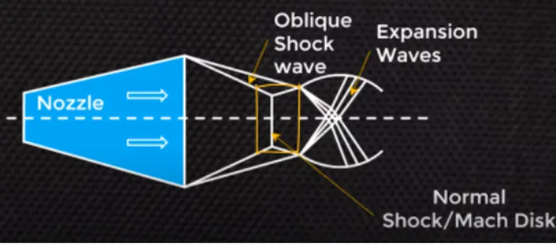
Shock waves are very thin on the order of magnitude of the mean free molecule path. Thus in the continuum description of gas dynamic, they are treated as discontinuities. Shock wave are characterized by an abrupt change of flow properties such as pressure, temperature, density, and a decrease in Mach number and total pressure, also an increase in entropy.
Geometry setup:
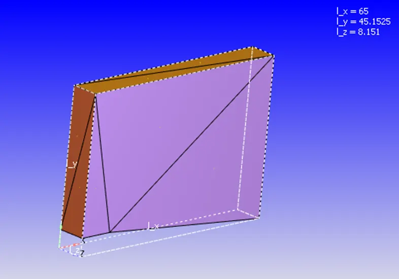
Case setup:
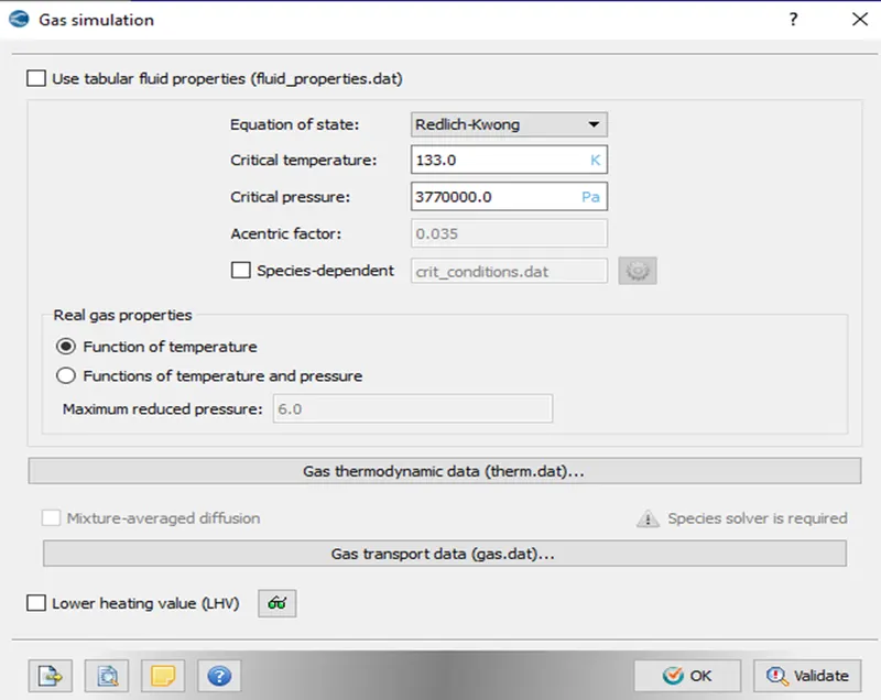
Gas simulation:
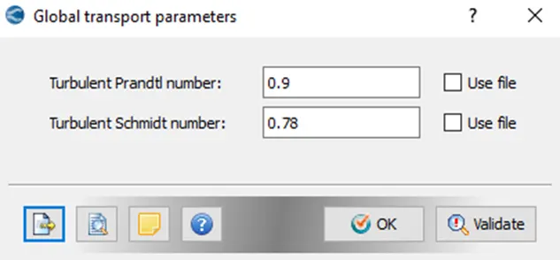
Global transport parameters:
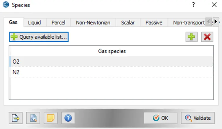
Species:
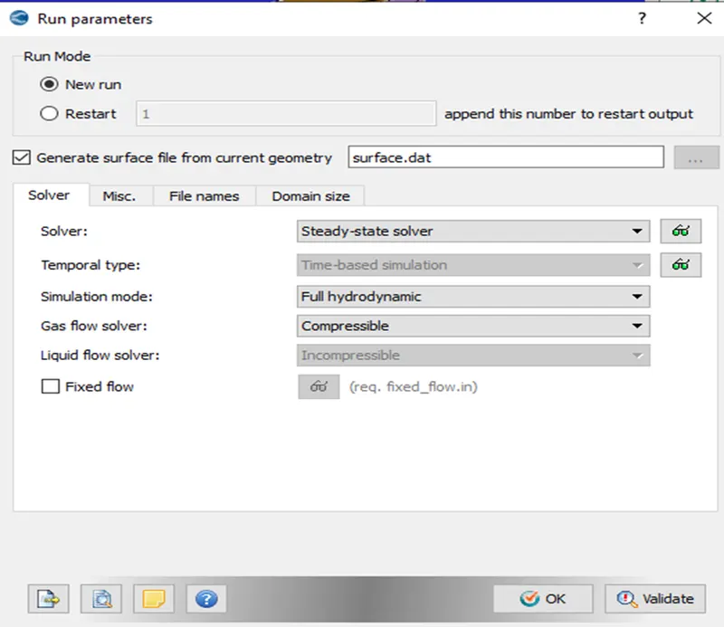
Run parameters:
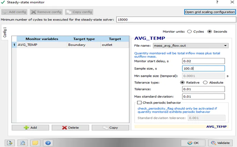
Steady state monitor:
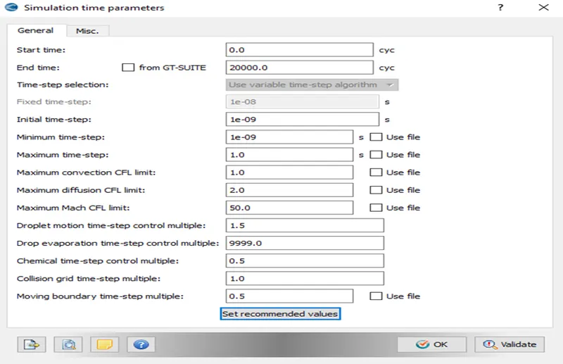
Simulation time parameters:
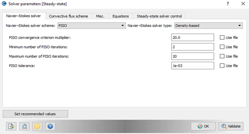
Solver parameters [steady-state]:
Boundary:
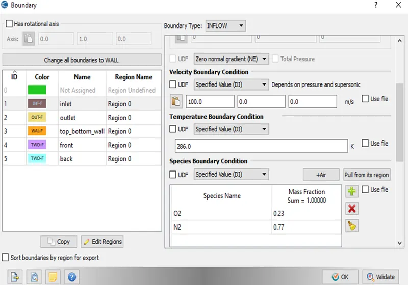
Inlet:
Velocity = 680 m/s.
Temperature = 286 K.
Species = Air.
Outlet:
Pressure = zero normal gradient.
Velocity = zero normal gradient.
Front and Back:
TWO-D
Top and bottom wall:
Slip wall
Simulation time parameters:
Start time: 0 cycle.
End time; 200000 cycle.
Solver: Density based steady state solver.
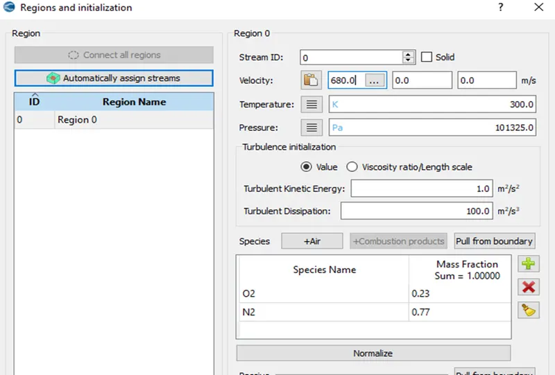
Fluid under consideration: Air (O2 + N2).
Regions and initialization:
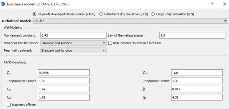
Turbulence modeling [RANS_K_EPS_RNG]:
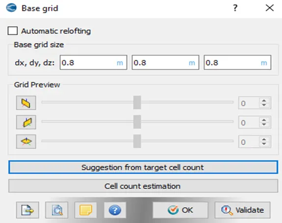
Base grid:
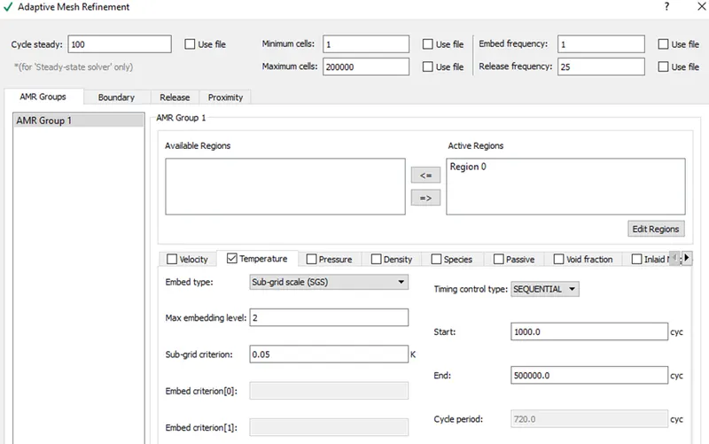
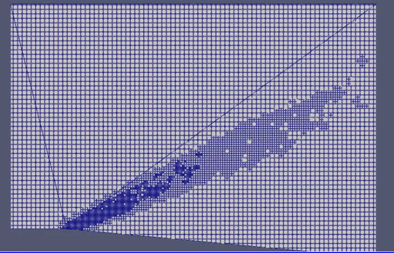
Adaptive mesh refinement:
Cases:
- Velocity = 680 m/s and SGS Temperature sub-grid criteria = 0.1.
- Velocity = 680 m/s and SGS Temperature sub-grid criteria = 0.05.
- Velocity = 100 m/s and SGS Temperature sub-grid criteria = 0.05.
Results:
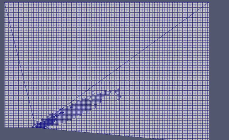
Case 1: Velocity = 680 m/s and SGS Temperature sub-grid criteria = 0.1.
Mesh:
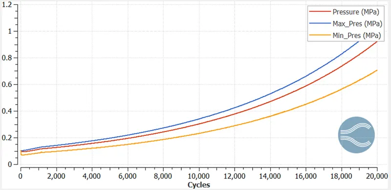
Pressure:
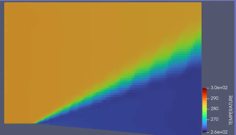
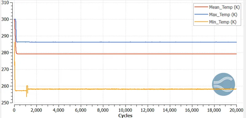
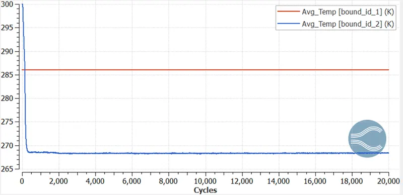
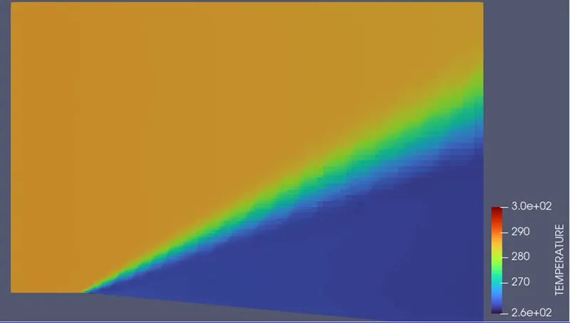
Temperature:
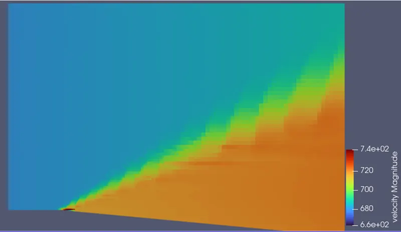
Velocity:
Total cell:
Case 2: Velocity = 680 m/s and SGS Temperature sub-grid criteria = 0.05.
Mesh:
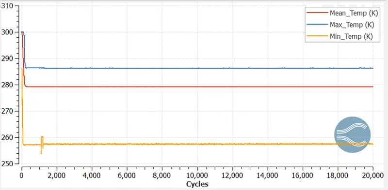
Temperature:
https://youtu.be/AA2aa5jMeT4
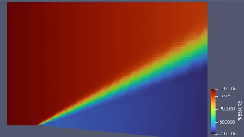
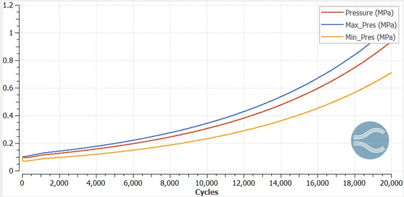
Pressure:
https://youtu.be/eIZLkpKdIZc
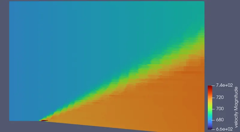
Velocity:
https://youtu.be/LfqVz-93LTE
Total cell count:
Density:
https://youtu.be/flXIkLqLayQ
Case 3: Velocity = 100 m/s and SGS Temperature sub-grid criteria = 0.05.
Mesh:
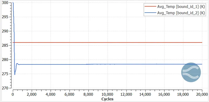
Temperature:
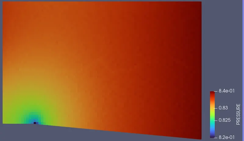
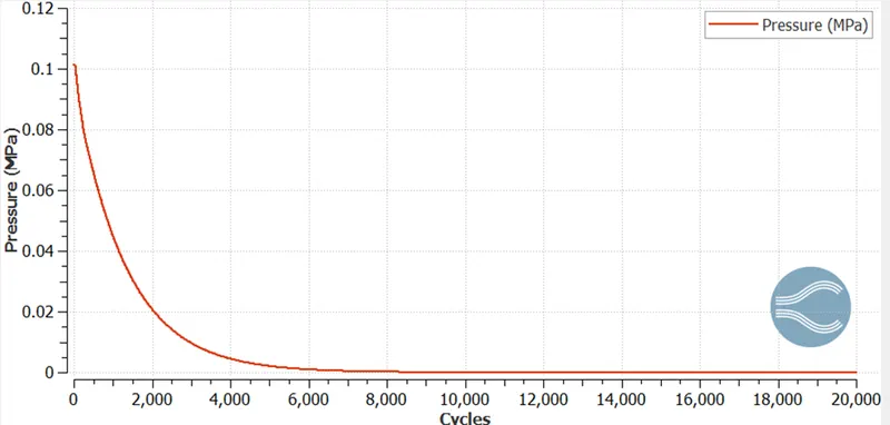
Pressure:
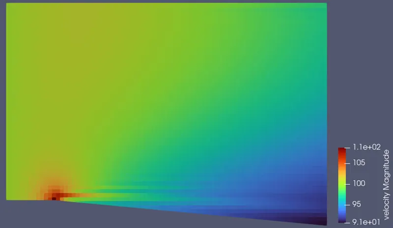
Velocity:
Effect on cell count:
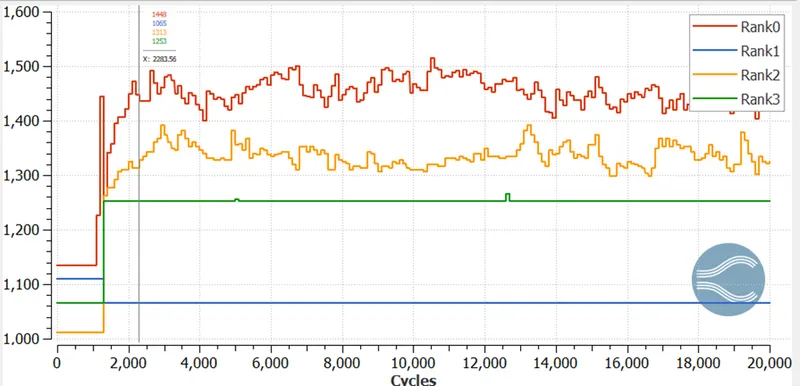
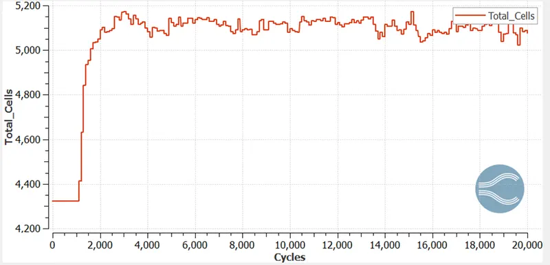
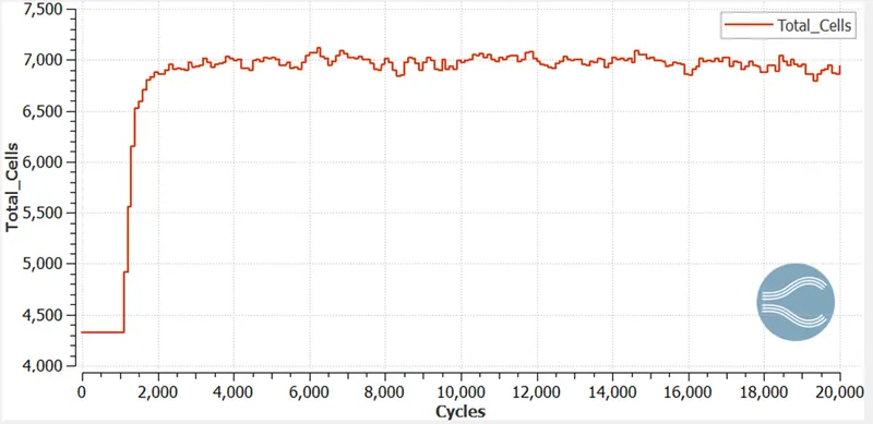
Form the above graph, the simulation with the least SGS value had the largest number of cell count. This is understandable because lower SGS ensures higher refinements results in higher of cells. For SGS =0.1. The refinement criteria were so higher that no refinements was achieved, it was as good as no adaptive mesh refinement.
Conclusion:
We were able to design a geometry with an expansion corner, simulate flow over and study the effects of SGS parameters. This can be beneficial when we design aircrafts that travel in supersonic speeds. We can simulate flow over various design and modify the expansion corners in the design such that the expansion wave does not affect the airflow around the aircraft.