Week 8- Moving zones approach in Fluent

Aim:

• To model moving zones for rotary equipments.
• To apply and understand different types of moving zones approach.

Take away:

After reading this article, one will be able to,

• Differentiate and apply different methods of moving zones to appropriate application.
• Apply moving reference frame approach to a particular type of problem.

===============================================================================

Overview of Moving Reference Frame:

Problems that involve multiple moving parts cannot be modeled with the Single Reference Frame approach. For these problems, you must break up the model into multiple fluid/solid cell zones, with interface boundaries separating the zones.

Zones that contain the moving components can then be solved using the moving reference frame equations, whereas stationary zones can be solved with the stationary frame equations.

The manner in which the equations are treated at the interface lead to two approaches:

1) Multiple Moving Reference Frame:

- Multiple Reference Frame model (MRF).

- Mixing Plane Model (MPM)

2) Sliding Mesh or Moving Mesh.

Both the MRF and mixing plane approaches are steady-state approximations, and differ primarily in the manner in which conditions at the interfaces are treated.

The sliding mesh model approach is, on the other hand, inherently unsteady due to the motion of the mesh with time.

Multiple Reference Frame model (MRF):

The MRF model is, perhaps, the simplest of the two approaches for multiple zones. It is a steady-state approximation in which individual cell zones can be assigned different rotational and/or translational speeds.

The flow in each moving cell zone is solved using the moving reference frame equations. If the zone is stationary (`omega` = 0), the equations reduce to their stationary forms.

At the interfaces between cell zones, a local reference frame transformation is performed to enable flow variables in one zone to be used to calculate fluxes at the boundary of the adjacent zone.

It should be noted that the MRF approach does not account for the relative motion of a moving zone with respect to adjacent zones (which may be moving or stationary); the mesh remains fixed for the computation. This is analogous to freezing the motion of the moving part in a specific position and observing the instantaneous flow field with the rotor in that position. Hence, the MRF is often referred to as the “frozen rotor approach.”

While the MRF approach is clearly an approximation, it can provide a reasonable model of the flow for many applications. For example, the MRF model can be used for turbomachinery applications in which rotor-stator interaction is relatively weak, and the flow is relatively uncomplicated at the interface between the moving and stationary zones. In mixing tanks, since the impeller-baffle interactions are relatively weak, large-scale transient effects are not present and the MRF model can be used.

Another potential use of the MRF model is to compute a flow field that can be used as an initial condition for a transient sliding mesh calculation. This eliminates the need for a startup calculation. The multiple reference frame model should not be used, however, if it is necessary to actually simulate the transients that may occur in strong rotor-stator interactions, as the sliding mesh model alone should be used.

Sliding Mesh Model:

The sliding mesh model is a special case of general dynamic mesh motion wherein the nodes move rigidly in a given dynamic mesh zone. Additionally, multiple cells zones are connected with each other through non-conformal interfaces.

As the mesh motion is updated in time, the non-conformal interfaces are likewise updated to reflect the new positions each zone. It is important to note that the mesh motion must be prescribed such that zones linked through non-conformal interfaces remain in contact with each other (that is,“slide” along the interface boundary) if you want fluid to be able to flow from one mesh to the other. Any portion of the interface where there is no contact is treated as a wall.

Reference: Ansys Fluent Guide.

==============================================================================

Simulation Procedure:

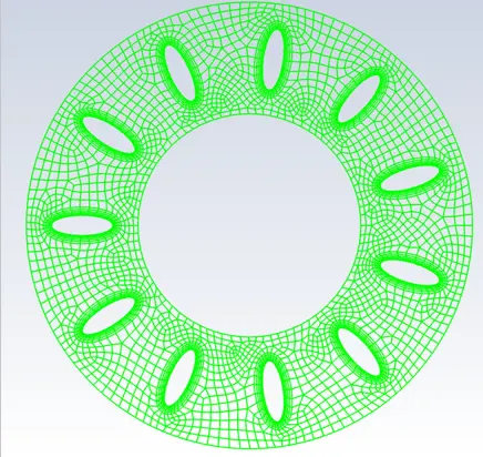
• Import the given geometry file into ansys fluent. As shown below:

General Settings:

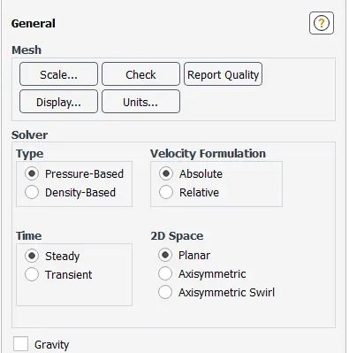
• It is steady state pressure based problem.

Viscous Model:

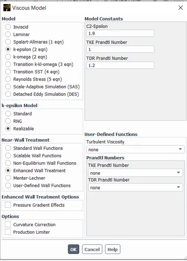
• k-epsilon realizable model with enhanced wall functions. Proven to give more accurate results compared to standard k-epsilon model.

Cell Zone Conditions:

• Here one must define the rotating parameters like for example, rpm of the rotor domain etc.

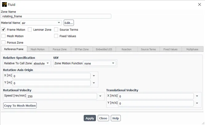
• Enable frame motin to mimic or capture rotation of blades.
• In this method the mesh does not move and hence it is a steady state approach.

Boundary Conditions:

• In this particular problem there is no inlet and outlet.
• But one must tell Ansys that walls of the blade are moving too.

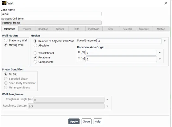
• Rev/min is zero with reference to 'Adjacent call zone'. We want the relative speed to be 0 between the walls of airfoil and the moving zone. This essentially tells that the blades are moving with the moving zone.

Methods:

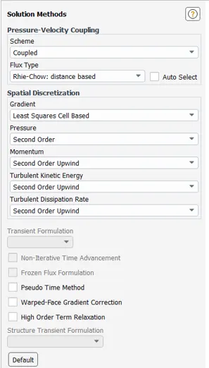
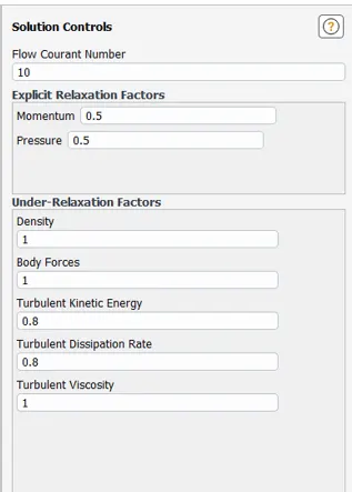
Control:

Initialization:

• Hybrid initialization.
• Run the simulation untill it converges.

==============================================================================

Results:

• Residuals:

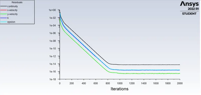
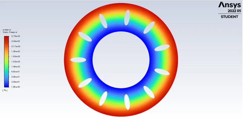
• Pressure Contour:

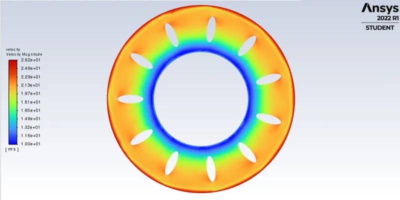
• Velocity Contour:

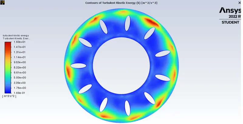
• Turbulent Kinitic Energy:

==============================================================================