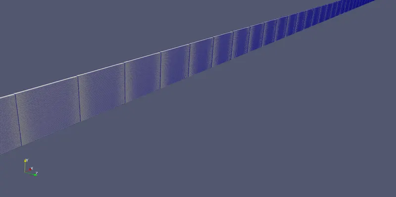
Week 11 - Simulation of Flow through a pipe in OpenFoam
Problem Statement:
Simulate flow through circular pipe and validate the results with Hagen Poiseuille equations (Hegen Poiseuille Law).
Given Condition:
- The flow is considered to be laminar.
- The value for Reynolds Number is considered to be 2100. In order for flow to be laminar Re < 2400.
- To save computational time, use of WEDGE boundary condition is done.
- blockMeshDict file must be created using MATLAB.
Brief understanding of Hagen Poiseuille equations:
Assumptions:
- The flow is considered to be incompressible.
- Fluid is Newtonian fluid; fluid which follows the Newton's Law viscosity.
- There is no slip of fluid near the wall of the pipe. Meaning the fluid comes to rest or the velocity of fluid is 'zero' near the walls of the pipe. It then tries to slow down the adjecent fluid layer. In order to compensate the velocity loss, the fluid velocity at the centerline of the pipe is is maximum and this phenomenon developes something called as velocity gradient.
The idea behinde the Hagen Poiseuille Law is that it gives the pressure drop in an incompressible and Newtonian fluid flowing through the circular pipe.
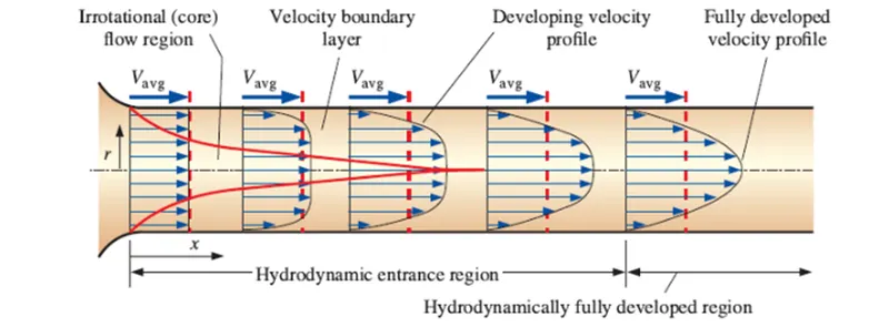
Diagram of flow through circular pipe:
Hydrodynamic Length:
- Entrance length refers to the length of the entry region, the area following the pipe entrance where effects originating from the interior wall of the pipe propagate into the flow as an expanding boundary layer.
- When the boundary layer expands to fill the entire pipe, the developing flow becomes a fully developed flow, where flow characteristics no longer change with increased distance along the pipe.
- Hydrodynamic entrance length describes the formation of a velocity profile caused by viscous forces propagating from the pipe wall.
- It is important to know the entrance length for effective working of instrument.
Equations of Hagen Poiseuille Flow:
- Average Velocity:
`V_(avg) = (Re*mu)/(rho*L_c)`
Re = Reynolds Number
`mu` = dynamic Viscosity
`rho` = Density of Fluid
L_c = Characteristic Length (our case = Diameter of pipe)
- Maximum Velocity:
`V_(max) = 2* V_(avg)`
- Pressure Drop:
`trianglep = (8*mu*V_(avg)*L)/(R^2)`
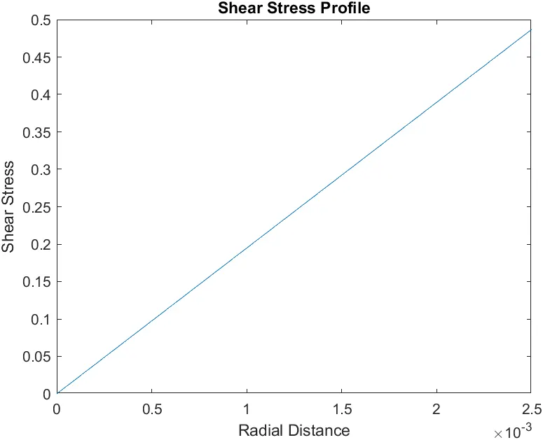
- Shear Stress:
`tau = (2*mu*V_(max)*R)/r^2`
R = range for radial distance.
r = radius of the pipe.
- Hydrodynamic Length:
`L_(enter) = 0.0575*Re*D`
==============================================================================
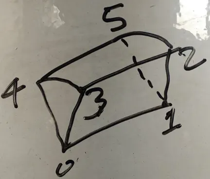
Geometry:
==============================================================================
blockMeshDict file generation using MATLAB:
CODE:
% blockMeshDict File creation

% Assumptions
Re = 2100; % Reynolds Number
D = input('Enter the Diameter of pipe: ');
% D = 0.005; % Diameter of pipe
r = D/2; % Radius of pipe
mu = 0.00085; % Dynamic Viscosity of water
rho = 997; % Density of water
theta = input('Enter the value of angle: ');
% theta = 4; % angle of the sector
% Entrance Length
L_enter = 0.0575*Re*D;
% Total Length of pipe
L_pipe = L_enter + 0.4;
% Hagen- Poiseuille's equations

% Average Velocity
v_avg = (Re*mu)/(rho*D);

% Maximum Velocity
v_max = 2*v_avg;

% Pressure Drop
p = (8*mu*v_avg*D)/(r^2);
kinematic_p = p/rho;

% Shear Stress Distribution from 0 to D/2
R = linspace(0,D/2,500);
for i = 1:length(R)
    tau(i) = (2*mu*v_max*(R(i)))/(r^2);
end

% Construction of blockMeshDict
f1 =  fopen('blockMeshDict','w');
head1 = '/*--------------------------------*- C++ -*----------------------------------*\';
head2 = '| =========                 |                                                 |';
head3 = '| \\      /  F ield         | OpenFOAM: The Open Source CFD Toolbox           |';
head4 = '|  \\    /   O peration     | Version:  v2012                                 |';
head5 = '|   \\  /    A nd           | Website:  www.openfoam.com                      |';
head6 = '|    \\/     M anipulation  |                                                 |';
head7 = '\*---------------------------------------------------------------------------*/';
fprintf(f1,'%s\n',head1);
fprintf(f1,'%s\n',head2);
fprintf(f1,'%s\n',head3);
fprintf(f1,'%s\n',head4);
fprintf(f1,'%s\n',head5);
fprintf(f1,'%s\n',head6);
fprintf(f1,'%s\n',head7);

fprintf(f1,'%s\n','FoamFile')
fprintf(f1,'%s\n','{')
fprintf(f1,'%10s \t 2.0;\n','version')
fprintf(f1,'%9s \t ascii;\n','format')
fprintf(f1,'%8s \t dictionary;\n','class')
fprintf(f1,'%9s \t blockMeshDict;\n','object')
fprintf(f1,'%s\n','}')

head8= '// * * * * * * * * * * * * * * * * * * * * * * * * * * * * * * * * * * * * * //';
fprintf(f1,'%s\n\n',head8);
fprintf(f1,'%s \t 1;\n\n','scale');
fprintf(f1,'%s\n','vertices')
fprintf(f1,'%s\n','(')
fprintf(f1,'\t (%d %d %d)\n',0,0,0); %0
fprintf(f1,'\t (%d %d %d)\n',L_pipe,0,0); %1
fprintf(f1,'\t (%d %d %d)\n',L_pipe,r*cosd(theta/2),r*sind(theta/2)); %2
fprintf(f1,'\t (%d %d %d)\n',0,r*cosd(theta/2),r*sind(theta/2)); %3
fprintf(f1,'\t (%d %d %d)\n',0,r*cosd(theta/2),-r*sind(theta/2)); %4
fprintf(f1,'\t (%d %d %d)\n',L_pipe,r*cosd(theta/2),-r*sind(theta/2)); %5
fprintf(f1,'%s\n\n',');');
fprintf(f1,'%s\n','blocks');
fprintf(f1,'%s\n','(');
x_mesh = input('Number of Mesh in X-Direction: ');
y_mesh = input('Number of Mesh in Y-Direction: ');
z_mesh = input('Number of Mesh in Z-Direction: ');
x_sg = input('Simple Grading in X-Direction: ');
y_sg = input('Simple Grading in Y-Direction: ');
z_sg = input('Simple Grading in Z-Direction: ');
fprintf(f1,'\t hex (%d %d %d %d %d %d %d %d) (%d %d %d) simpleGrading (%d %d %d)\n',0,1,5,4,0,1,2,3,x_mesh,y_mesh,z_mesh,x_sg,y_sg,z_sg);
fprintf(f1,'%s\n\n',');');
fprintf(f1,'%s \n','edges');
fprintf(f1,'%s\n','(');
fprintf(f1,'\t arc %d %d (%d %d %d)\n',3,4,0,r,0);
fprintf(f1,'\t arc %d %d (%d %d %d)\n',2,5,L_pipe,r,0);
fprintf(f1,'%s \n\n',');');
fprintf(f1,'%s \n','boundary');
fprintf(f1,'%s \n','(');
% Defining Inlet
fprintf(f1,'\t %s \n','inlet');
fprintf(f1,'\t %s \n','{');
fprintf(f1,'\t\t %s %s \n','type','patch;');
fprintf(f1,'\t\t %s \n','faces');
fprintf(f1,'\t\t %s \n','(');
fprintf(f1,'\t\t\t (%d %d %d %d) \n',0,3,4,0);
fprintf(f1,'\t\t %s \n',');');
fprintf(f1,'\t %s \n','}');

% Defining Outlet
fprintf(f1,'\t %s \n','outlet');
fprintf(f1,'\t %s \n','{');
fprintf(f1,'\t\t %s %s \n','type','patch;');
fprintf(f1,'\t\t %s \n','faces');
fprintf(f1,'\t\t %s \n','(');
fprintf(f1,'\t\t\t (%d %d %d %d) \n',1,5,2,1);
fprintf(f1,'\t\t %s \n',');');
fprintf(f1,'\t %s \n','}');

% Defining Top
fprintf(f1,'\t %s \n','top');
fprintf(f1,'\t %s \n','{');
fprintf(f1,'\t\t %s %s \n','type','wall;');
fprintf(f1,'\t\t %s \n','faces');
fprintf(f1,'\t\t %s \n','(');
fprintf(f1,'\t\t\t (%d %d %d %d) \n',3,4,5,2);
fprintf(f1,'\t\t %s \n',');');
fprintf(f1,'\t %s \n','}');

% Defining Front
fprintf(f1,'\t %s \n','front');
fprintf(f1,'\t %s \n','{');
fprintf(f1,'\t\t %s %s \n','type','wedge;');
fprintf(f1,'\t\t %s \n','faces');
fprintf(f1,'\t\t %s \n','(');
fprintf(f1,'\t\t\t (%d %d %d %d) \n',0,1,2,3);
fprintf(f1,'\t\t %s \n',');');
fprintf(f1,'\t %s \n','}');

% Defining Back
fprintf(f1,'\t %s \n','back');
fprintf(f1,'\t %s \n','{');
fprintf(f1,'\t\t %s %s \n','type','wedge;');
fprintf(f1,'\t\t %s \n','faces');
fprintf(f1,'\t\t %s \n','(');
fprintf(f1,'\t\t\t (%d %d %d %d) \n',0,4,5,1);
fprintf(f1,'\t\t %s \n',');');
fprintf(f1,'\t %s \n','}');

% Defining Axis
fprintf(f1,'\t %s \n','axis');
fprintf(f1,'\t %s \n','{');
fprintf(f1,'\t\t %s %s \n','type','empty;');
fprintf(f1,'\t\t %s \n','faces');
fprintf(f1,'\t\t %s \n','(');
fprintf(f1,'\t\t\t (%d %d %d %d) \n',0,1,1,0);
fprintf(f1,'\t\t %s \n',');');
fprintf(f1,'\t %s \n','}');

fprintf(f1,'%s \n\n',');');
fprintf(f1,'%s \n','mergePatchPairs');
fprintf(f1,'%s \n','(');
fprintf(f1,'%s \n\n',');');
head9 = '// ************************************************************************* //';
fprintf(f1,'%s \n',head9);


% Analytical Results
figure(1)
plot(R,tau)
xlabel('Radial Distance')
ylabel('Shear Stress')
title('Shear Stress Profile')
figure(2)
for i = 1:length(R)
    u(i) = v_max*((abs((1 - ((R(i).^2)./(r)^2)))));
end
plot(R,u)
xlabel('Radial Distance')
ylabel('Velocity')
title('Velocity Profile')
blockMeshDict file output:
/*--------------------------------*- C++ -*----------------------------------*\
| =========                 |                                                 |
| \\      /  F ield         | OpenFOAM: The Open Source CFD Toolbox           |
|  \\    /   O peration     | Version:  v2012                                 |
|   \\  /    A nd           | Website:  www.openfoam.com                      |
|    \\/     M anipulation  |                                                 |
\*---------------------------------------------------------------------------*/
FoamFile
{
   version 	 2.0;
   format 	 ascii;
   class 	 dictionary;
   object 	 blockMeshDict;
}
// * * * * * * * * * * * * * * * * * * * * * * * * * * * * * * * * * * * * * //

scale 	 1;

vertices
(
	 (0 0 0)
	 (1.003750e+00 0 0)
	 (1.003750e+00 2.498477e-03 8.724874e-05)
	 (0 2.498477e-03 8.724874e-05)
	 (0 2.498477e-03 -8.724874e-05)
	 (1.003750e+00 2.498477e-03 -8.724874e-05)
);

blocks
(
	 hex (0 1 5 4 0 1 2 3) (300 50 1) simpleGrading (1 1 1)
);

edges
(
	 arc 3 4 (0 2.500000e-03 0)
	 arc 2 5 (1.003750e+00 2.500000e-03 0)
);

boundary
(
	 inlet
	 {
		 type patch;
		 faces
		 (
			 (0 3 4 0)
		 );
	 }
	 outlet
	 {
		 type patch;
		 faces
		 (
			 (1 5 2 1)
		 );
	 }
	 top
	 {
		 type wall;
		 faces
		 (
			 (3 4 5 2)
		 );
	 }
	 front
	 {
		 type wedge;
		 faces
		 (
			 (0 1 2 3)
		 );
	 }
	 back
	 {
		 type wedge;
		 faces
		 (
			 (0 4 5 1)
		 );
	 }
	 axis
	 {
		 type empty;
		 faces
		 (
			 (0 1 1 0)
		 );
	 }
);

mergePatchPairs
(
);

// ************************************************************************* //
==============================================================================
Pressure file p:
/*--------------------------------*- C++ -*----------------------------------*\
| =========                 |                                                 |
| \\      /  F ield         | OpenFOAM: The Open Source CFD Toolbox           |
|  \\    /   O peration     | Version:  v2012                                 |
|   \\  /    A nd           | Website:  www.openfoam.com                      |
|    \\/     M anipulation  |                                                 |
\*---------------------------------------------------------------------------*/
FoamFile
{
    version     2.0;
    format      ascii;
    class       volScalarField;
    object      p;
}
// * * * * * * * * * * * * * * * * * * * * * * * * * * * * * * * * * * * * * //

dimensions      [0 2 -2 0 0 0 0];

internalField   uniform 0;

boundaryField
{
    inlet
    {
        type            zeroGradient;
    }

    outlet
    {
        type            fixedValue;
	value		uniform 0;
    }

    top
    {
        type            zeroGradient;
    }

    front
    {
        type            wedge;
    }

    back
    {
        type            wedge;
    }

    axis
    {
        type            empty;
    }
}

// ************************************************************************* //
==============================================================================
Velocity file U:
/*--------------------------------*- C++ -*----------------------------------*\
| =========                 |                                                 |
| \\      /  F ield         | OpenFOAM: The Open Source CFD Toolbox           |
|  \\    /   O peration     | Version:  v2012                                 |
|   \\  /    A nd           | Website:  www.openfoam.com                      |
|    \\/     M anipulation  |                                                 |
\*---------------------------------------------------------------------------*/
FoamFile
{
    version     2.0;
    format      ascii;
    class       volVectorField;
    object      U;
}
// * * * * * * * * * * * * * * * * * * * * * * * * * * * * * * * * * * * * * //

dimensions      [0 1 -1 0 0 0 0];

internalField   uniform (1 0 0);

boundaryField
{
    inlet
    {
        type            fixedValue;
        value           uniform (0.3581 0 0);
    }

    outlet
    {
        type            zeroGradient;
    }

    top
    {
        type            fixedValue;
	value		uniform (0 0 0);
    }

    front
    {
        type            wedge;
    }

    back
    {
        type            wedge;
    }

    axis
    {
        type            empty;
    }
}

// ************************************************************************* //
==============================================================================
controlDict:
/*--------------------------------*- C++ -*----------------------------------*\
| =========                 |                                                 |
| \\      /  F ield         | OpenFOAM: The Open Source CFD Toolbox           |
|  \\    /   O peration     | Version:  v2012                                 |
|   \\  /    A nd           | Website:  www.openfoam.com                      |
|    \\/     M anipulation  |                                                 |
\*---------------------------------------------------------------------------*/
FoamFile
{
    version     2.0;
    format      ascii;
    class       dictionary;
    location    "system";
    object      controlDict;
}
// * * * * * * * * * * * * * * * * * * * * * * * * * * * * * * * * * * * * * //

application     icoFoam;

startFrom       startTime;

startTime       0;

stopAt          endTime;

endTime         1;

deltaT          0.001;

writeControl    timeStep;

writeInterval   20;

purgeWrite      0;

writeFormat     ascii;

writePrecision  6;

writeCompression off;

timeFormat      general;

timePrecision   6;

runTimeModifiable true;


// ************************************************************************* //
==============================================================================
transportProperties:
In transport properties one has to change the value of `nu` which is given by the formula: `nu = mu/rho`
/*--------------------------------*- C++ -*----------------------------------*\
| =========                 |                                                 |
| \\      /  F ield         | OpenFOAM: The Open Source CFD Toolbox           |
|  \\    /   O peration     | Version:  v2012                                 |
|   \\  /    A nd           | Website:  www.openfoam.com                      |
|    \\/     M anipulation  |                                                 |
\*---------------------------------------------------------------------------*/
FoamFile
{
    version     2.0;
    format      ascii;
    class       dictionary;
    location    "constant";
    object      transportProperties;
}
// * * * * * * * * * * * * * * * * * * * * * * * * * * * * * * * * * * * * * //

nu              8.5255e-7;


// ************************************************************************* //
==============================================================================
Validation of results:
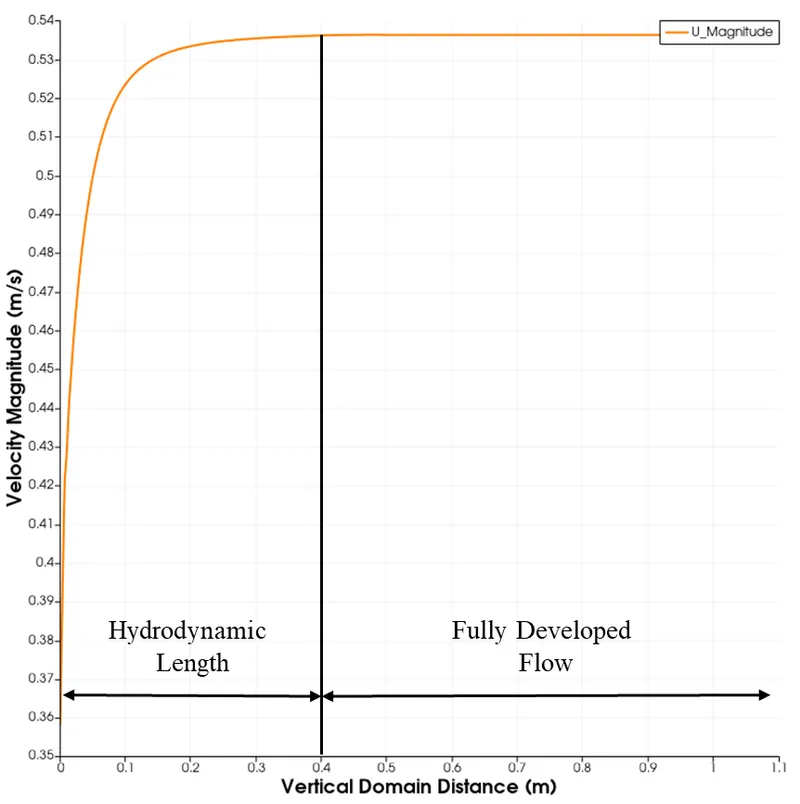
1) Hydrodynamic Length:
MATLAB Results:
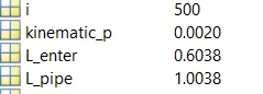
Points to take away:
- Entrance Region or hydrodynamic length is region where flow develops and is still not fully developed. It creates a velocity profile due to pipe wall force generation.
- Looking at the graph we can observe that after x = 0.4, the velocity is constant. We can say that the hydrodynamic length of the pipe is in between x= 0.4 or x = 0.5.
- The value of Entrance length obtaned from analytical solution is 0.6038 (L_enter in figure).
- It is close to what we have got from the simulation. The reason of not matching with analytical value is coarse mesh.
- Refining the mesh will bring the value closer to the analytical value.
|
Theoretical |
Simulation |
Error |
| 0.6038 | 0.4 | 33.75 % |
==============================================================================
2) Velocity Profile:
MATLAB Results:
Points to take away:
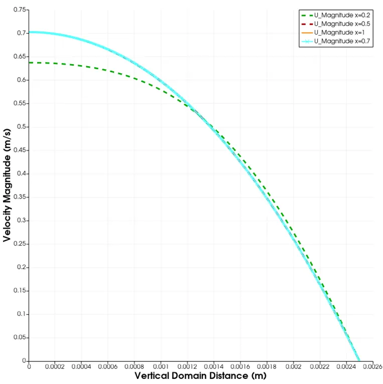
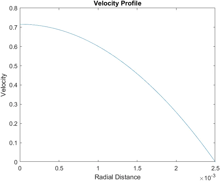
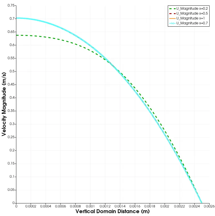
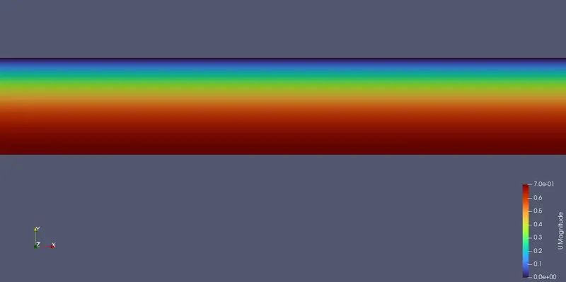
- The two figures depict the velocity profile along the radial direction at various x locations (x= 0.2,0.5,0.7,1).
- The profile at x= 0.2 lies inside the developing region of the flow.
- For x= 0.5,0.7,1, the flow is fully developed and it matches with the analytical solution. The figure below (MATLAB results) is the analytical solution and is given by the equation,
`V = V_(max)*[1-(r/R)^2]`
r is varying along the radius of the pipe and R is number of points along the radius of the pipe.
==============================================================================
3) Maximum Velocity and Pressure drop:
a) Maximum Velocity:
MATLAB Results:
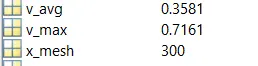
Points to take away:
|
Theoretical |
Simulation |
Error |
| 0.7161 | 0.7027 | 1.87 % |
b) Presseure Drop:
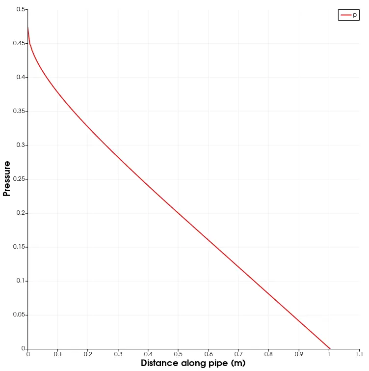
MATLAB Results:
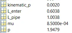
Points to take away:
Note: It is kinematic pressure and not pressure.
|
Theoretical |
Simulation |
Error |
| 0.0020 | 0.0023 | 15 % |
- This kinematic pressure is at the end the pipe length.
- The error can be reduced by increasing the mesh count. (refining the mesh).
==============================================================================
4) Shear Stress:
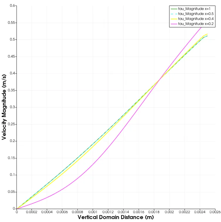
MATLAB Results:
Points to take away:
- At x = 0.2, inside the developing flow region the shear stress is not linear which what is expected due to the no slip condition near the wall.
- As we proceed along the length, the shear stress profile pretty much linearizes which is what is expected as it is in the fully developed region.
==============================================================================
Contours:
1) Velocity:
2) Mesh: