Week 8 - Simulating Cyclone separator with Discrete Phase Modelling

Aim: To perform a simulation on cyclone separator and understand how particles are separated.

Objective:

• To carry out a CFD simulation on cyclone separator.
• Effect of different particle size seperation efficiency with constant velocity.
• Effect of different velocities on same particle size separation efficiency.
• Understand pressure drop due to different velocity.

Problem Statement:

1. To write a few words about any four empirical models used to calculate the cyclone separator efficiency.
2. To perform an analysis on a given cyclone separator model by varying the particle diameter from 1 μm to 5 μm and calculate the separation efficiency in each case. Discuss the results. [Use both the velocity's as 3m/sec.]
3. To perform an analysis on a given cyclone separator model by varying the particle velocity from 1 m/sec to 5 m/sec and calculate the separation efficiency and pressure drop in each case. Discuss the results. [Use particle diameter size as 5 μm for all cases & keep flow velocity same as particle velocity]

Boundary Conditions:-

Inlet and wall:- Reflect

Outlet(Top):- Escape

Outlet(Bottom/dustbin) - Trap

==============================================================================

What is cyclone separator?

• Cyclonic separation is a method of removing particulates from an air, gas or liquid stream, without the use of filters, through vortex separation.
• When removing particulate matter from liquid, a hydrocyclone is used; while from gas, a gas cyclone is used.
• Rotational effects and gravity are used to separate mixtures of solids and fluids. The method can also be used to separate fine droplets of liquid from a gaseous stream.

Working:

• A high speed rotating (air)flow is established within a cylindrical or conical container called a cyclone.
• Air flows in a helical pattern, beginning at the top (wide end) of the cyclone and ending at the bottom (narrow) end before exiting the cyclone in a straight stream through the center of the cyclone and out the top.
• Larger (denser) particles in the rotating stream have too much inertia to follow the tight curve of the stream, and thus strike the outside wall, then fall to the bottom of the cyclone where they can be removed.
• In a conical system, as the rotating flow moves towards the narrow end of the cyclone, the rotational radius of the stream is reduced, thus separating smaller and smaller particles.
• The cyclone geometry, together with volumetric flow rate, defines the cut point of the cyclone.
• This is the size of particle that will be removed from the stream with a 50% efficiency.
• Particles larger than the cut point will be removed with a greater efficiency, and smaller particles with a lower efficiency as they separate with more difficulty or can be subject to re-entrainment when the air vortex reverses direction to move in direction of the outlet.

Empirical Models:

1. Iozia and Leith Model:

• This model is based on force balance.
• The model assumes that a particle carried by the vortex endures the influence of two forces: a centrifugal force, Z and a flow resistance, W.
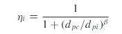
• The collection efficiency `eta_i` of a particle diameter dpi can be calculated as,

• β is an expression for slope parameter derived based on thestatistical analysis of experimental data of a cyclone with D = 0.25 m given as,

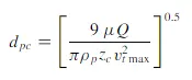
• dpc is given by,

• where core length, zc, and core diameter, dc, are given as,

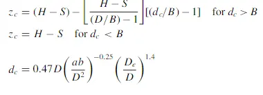
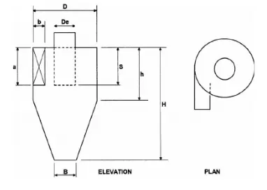
• Values of H, S, B etc can be taken from diagram,

2. Li and Wang Model:

• This model includes particle bounce or re-entrainment and turbulent diffusion at the cyclone wall.
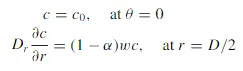
• A two-dimensional analytical expression of particle distribution in the cyclone is obtained. Li and Wang model was developed based on the following assumptions:

• The tangential velocity is related to the radius of cyclone by: `uR^n`= constant.
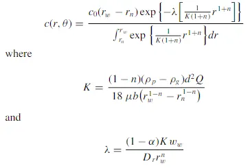
• The concenntration distribution in cyclone is given as:

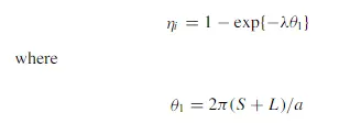
• The resultant expression of the collection efficiency for particle of any size is given as:

3. Koch and Licht Model:

• This collection theory recognized the inherently turbulent nature of cyclones and the distribution of gas residence times within the cyclone.
• Koch and Licht described particle motion in the entry and collection regions with the additional following assumptions:

-- The tangential velocity of a particle is equal to the tangential velocity of the gas flow, i.e. there is no slip in the tangential direction between the particle and the gas.

-- The tangential velocity is related to the radius of cyclone by: `uR^n`= constant.

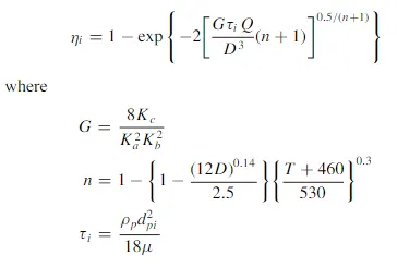
• A force balance and an equation on the particles collection yields the grade efficiency, `eta_i`

• G is a factor related to the configuration of the cyclone, n isrelated to the vortex and τ is the relaxation term.

4. Lapple Model:

• Lapple [1] model was developed based on force balance without considering the flow resistance.
• Lapple assumed that a particle entering the cyclone is evenly distributed across the inlet opening.
• The particle that travels from inlet half width to the wall in the cyclone is collected with 50% efficiency.
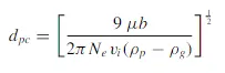
• The semi empirical relationship developed by Lapple to calculate a 50% cut diameter, dpc, is:

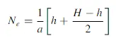
• where Ne is the number of revolutions,

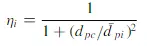
• The efficiency of collection of any size of particle is given by,

Reference : Link

==============================================================================

Simulation Procedure:

The simmulation was carried out in two parts each having 5 cases.

Part 1: With varying particle diameter.

Part 2: With varying the velocity.

==============================================================================

Part 1: Varying the particle diameter from `1mum` to `5mum` and velocity = 3m/s.

Case 1: `5mum`

Creating Geometry:

• Load the provided model into spaceclaim.
• Go to volume extract option and select edge selection.
• Select the inlet edge, outlet edge (top and bottom both) and hit the green tick mark to create the volume.
• Make sure to supress the solid body and keep just the extracked volume.

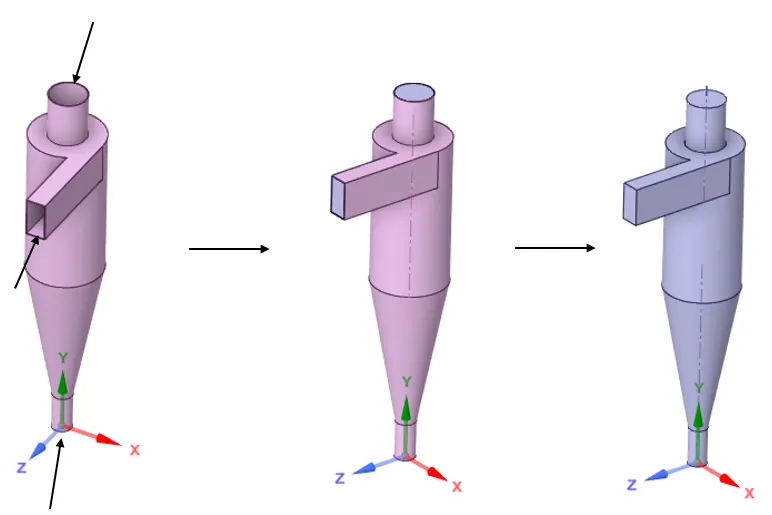
• The geometry is ready for meshing.
• The above procedure for geometry creation is same for all the cases.

Meshing:

• Set the global element size to 6 mm. (free choice)
• Right click on mesh and select 'methods' option.
• Select 'Cartesian' for methods and generate the mesh.
• This is the cutcell method which generates hexahedral mesh.

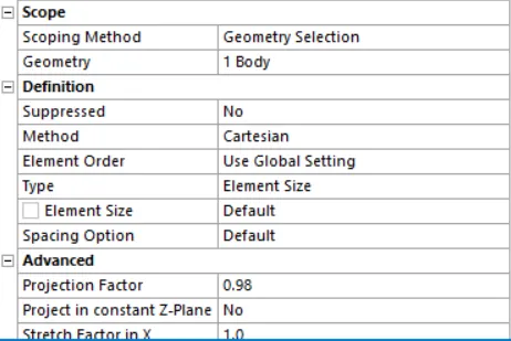
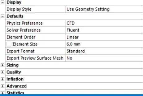
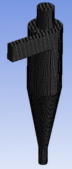
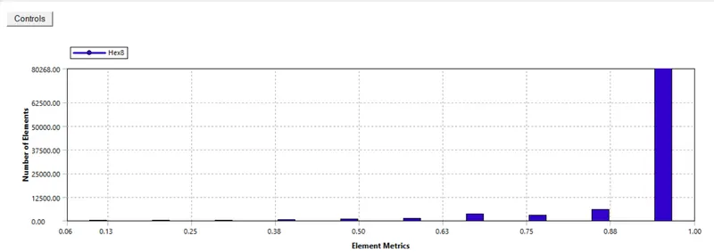
• The mesh setup is same for all the cases.

Setting up the Physics:

• Viscous Model: k-epsilon RNG Swirl Dominanted Flow, this gives a better approximaiton for flows with swirls.

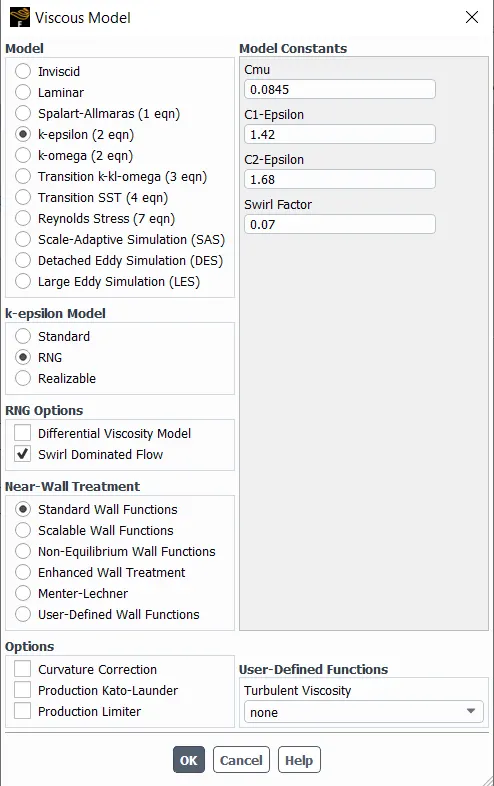
• Select Discrete Phase model.
• Select 'Interaction with Continuous Phase'. This allows the interaction between the continuous phase and the particles.
• Continuous phase is the fluid and the discrete phase is the particle to be separated (in this case).

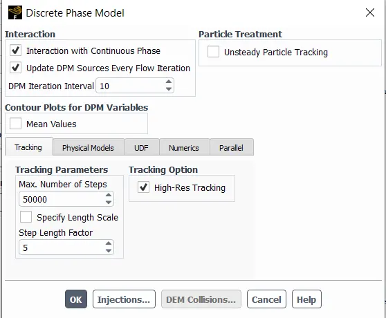
• Select 'Injections'.
• Set 'Injection type' to surface and select inlet.
• Assign 3 m/s in x-direction.
• One can use the 'Inject using Face Normal Direction', this assures that the velocity is normal to the surface selected.

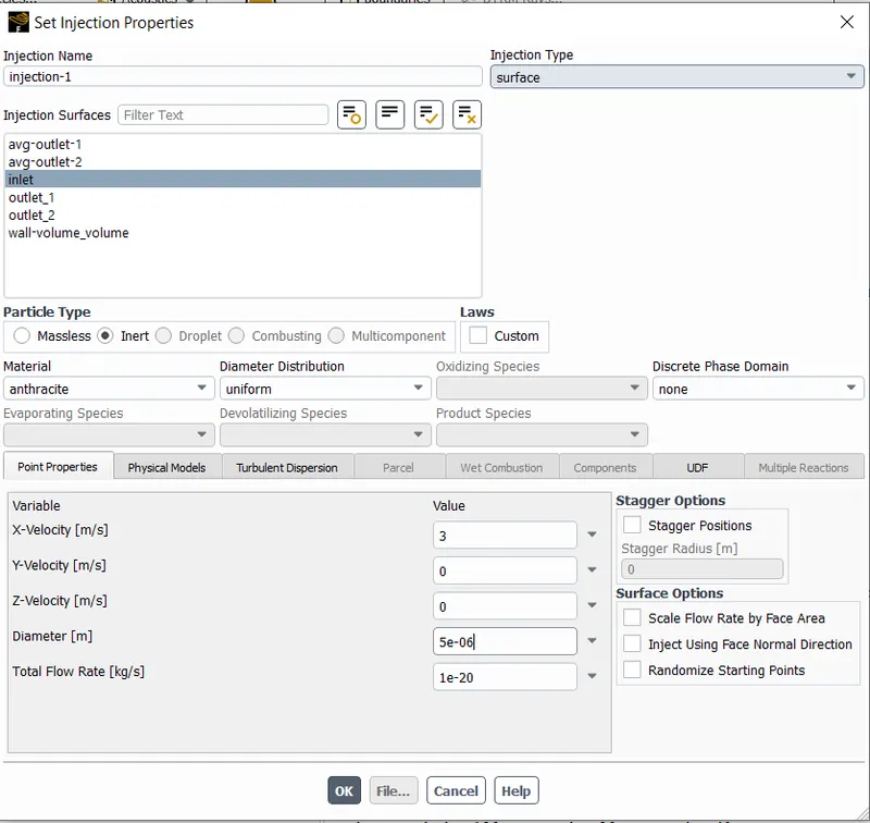
• For diameter assign 5e-06 m. This is for Case 1 of Part 1.
• Therefore, the only change in the other cases of part 1 is the Diameter of particle.
• Part 1 Case 1, Diameter = 5e-06
• Part 1 Case 2, Diameter = 4e-06
• Part 1 Case 3, Diameter = 3e-06
• Part 1 Case 4, Diameter = 2e-06
• Part 1 Case 5, Diameter = 1e-06

• Select the boundaries option.
• For inlet:

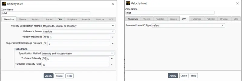
• For top outlet:

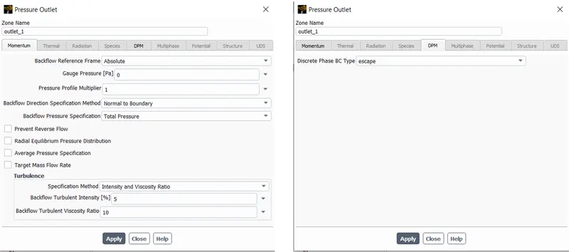
• For bottom outlet:

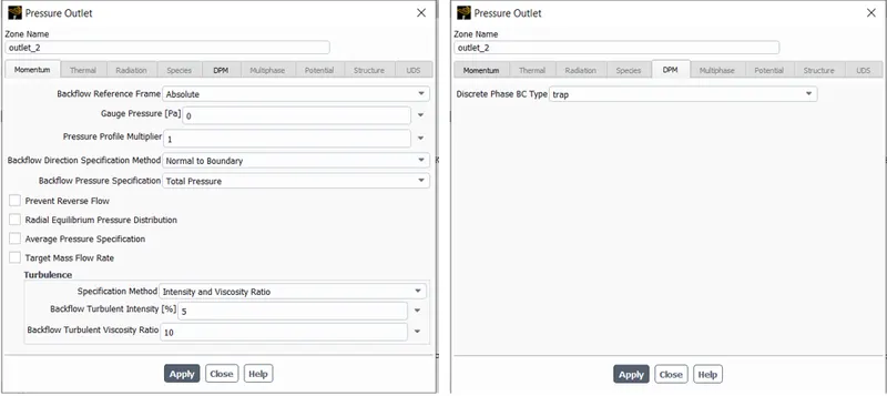
• For wall:

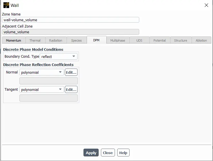
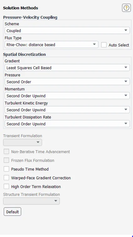
• Navigate to 'Methods' and set the following parameters to:

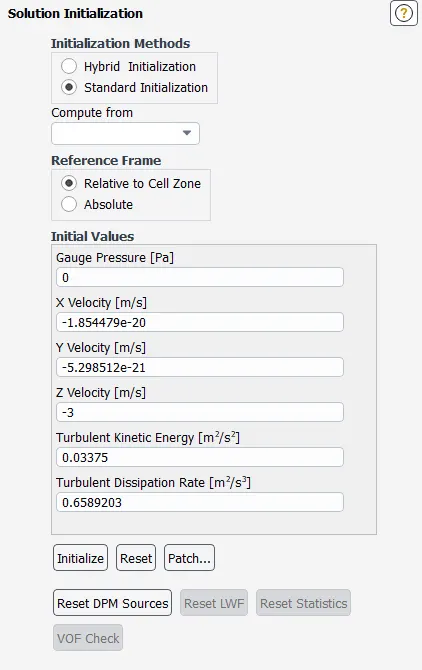
• Conduct a Standard Initialization.
• Compute from inlet.

• Give the number of iteraion and hit Run.

==============================================================================

Results for Part 1: (all the cases)

• Separation Efficiency = (Particles traped/ particles tracked)*100

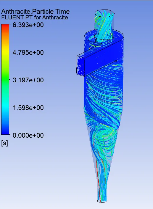
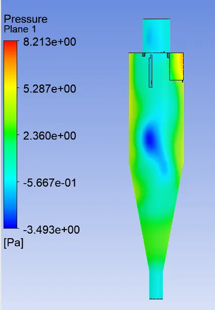
Case 1: `5 mum`

Separation Efficiency = (40/136)*100 = 29.411 %

• Particle Residence Time:

• Pressure Contour:

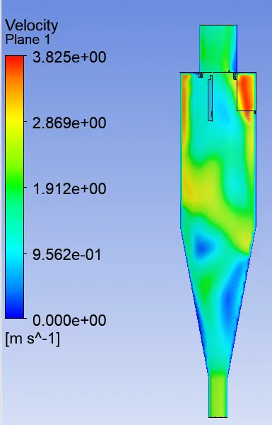
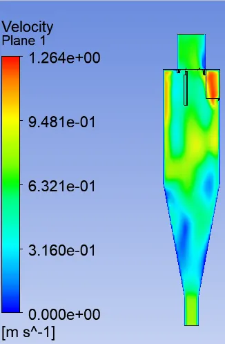
• Velocity Contour:

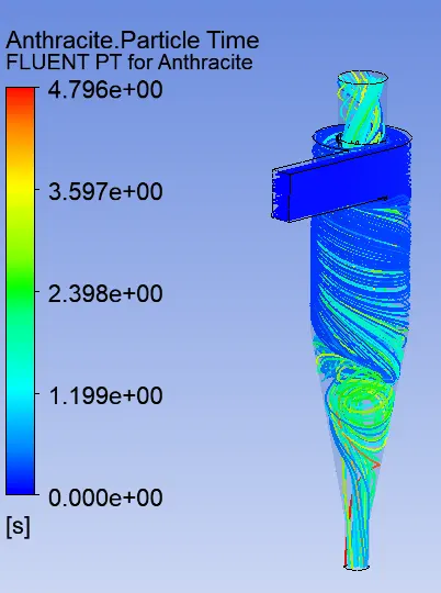
Case 2: `4mum`

Separation Efficiency = (48/136)*100 = 35.29%

• Particle Residence Time:

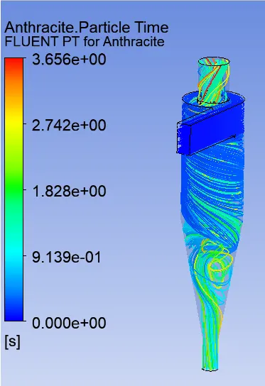
Case 3: `3mum`

Separation Efficiency = (49/136)*100 = 36.02%

• Particle Residence Time:

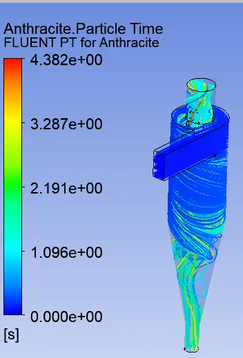
Case 4: `2mum`

Separation Efficiency = (28/136)*100 = 20.85 %

• Particle Residence Time:

Case 5: `1mum`

Separation Efficiency = (29/136)*100 = 21.32%

• Particle Residence Time:

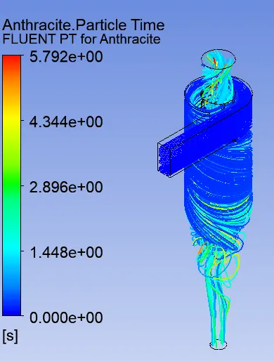
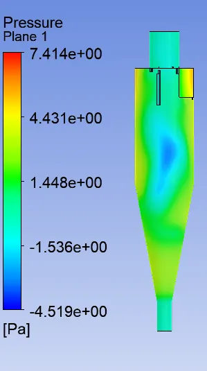
• Pressure and Velocity Contours are same for all the cases as the velocity is same for all the cases.

Conclusion:

• The efficiency increases upto particle diameter 3 micrometer and seperation efficiency is higher for 3 micrometer.
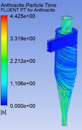
• The Residence time is highest for 5 micrometer.
• The results do not show consistency with respect to change in diameter.
• Therefore, furthur mesh refinement is necessary.

==============================================================================

Part 2: Varying the inlet velocity from 1m/s to 5m/s and keeping particle diameter constant.

• Everything is similar to Part 1, the only change is in the setup of discrete phase change tab.
• Instead of varying the particle diameter, we will vary the x-velocity.
• Note that in boundaries the velocity must be same as particle velocity. ie. x-velocity.

• Part 2,Case 1 = 5m/s
• Part 2,Case 2 = 4m/s
• Part 2,Case 3 = 3m/s
• Part 2,Case 4 = 2m/s
• Part 2,Case 5 = 1m/s

==============================================================================

Results for Part 2: (all cases)

Separation Efficiency = (Particle Traped/Particle Tracked)*100

Case 1: 5m/s

Separation Efficiency = (23/136)*100 = 16.911%

Pressure Drop = Total Inlet Pressure - Total Outlet Pressure

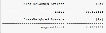
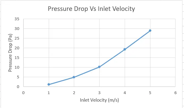
Pressure Drop = 33.3216 - 4.2932 = 29.0284 Pa

• Particle Residence Time:

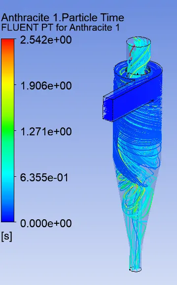
• Pressure Contour:

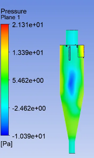
• Velocity Contour:

Case 2: 4m/s

Separatipn Efficiency = (24/136)*100 = 17.64%

Pressure drop = Total Inlet Pressure - Total Outlet Pressure

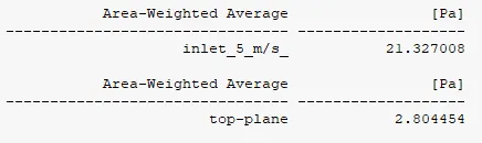
Pressure drop = 21.327 - 2.8044 = 19.2426 Pa

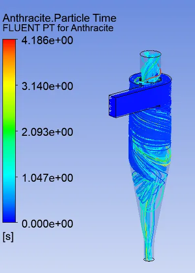
• Particle Residence Time:

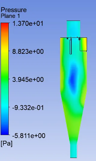
• Pressure Contour:

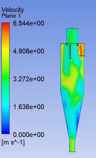
• Velocity Contour:

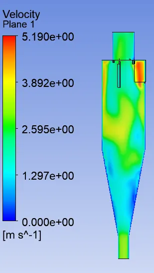
Case 3: 3 m/s

Separation Efficiency = (52/136)*100 = 38.23%

Pressure drop = Total Inlet Pressure - Total Outlet Pressure

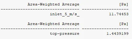
Pressure drop = 11.7445 - 1.4439 = 10.3006 Pa

• Particle Residence Time:

• Pressure Contour:

• Velocity Contour:

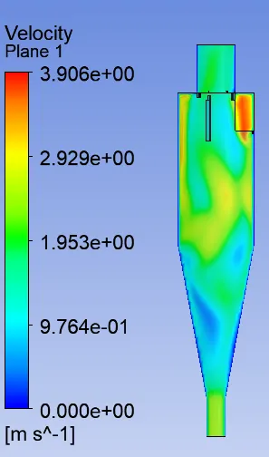
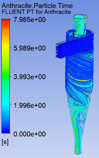
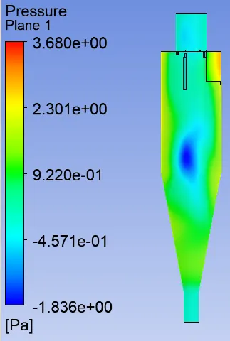
Case 4: 2m/s

Separation Efficiency = (35/136)*100 = 25.73%

Pressure drop = Total Inlet Pressure - Total Outlet Pressure

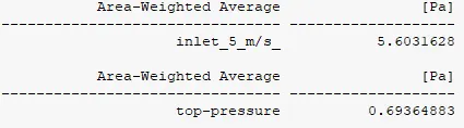
Pressure drop = 5.6031 - 0.6936 = 4.9097 Pa

• Particle Residence Time:

• Pressure Contour:

• Velocity Contour:

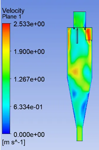
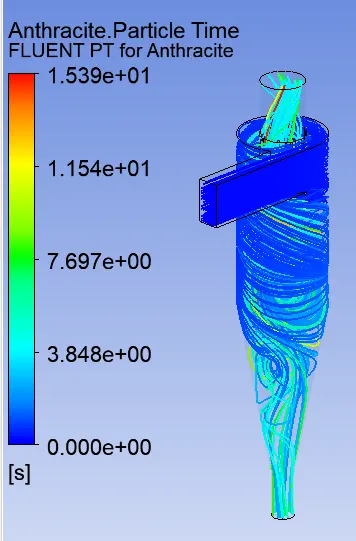
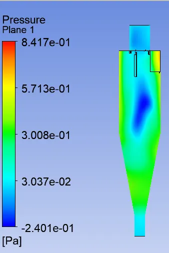
Case 5: 1m/s

Separation Efficiency = (31/136)*100 = 22.79%

Pressure drop = Total Inlet Pressure - Total Outlet Pressure

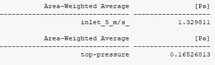
Pressure drop = 1.3298 - 0.1652 = 1.1646 Pa

• Particle Residence Time:

• Pressure Contour:

• Velocity Contour:

Conclusion:

• The highest separation efficiency is achieved for 3m/s case.
• The mesh needs to be more finer so that we can have more particles.
• The pressure drop increases with increase in velocity.

Paper: