Week 5 - Turbulence modelling challenge

Aim:

• To understand what is turbulence and how it can be modelled mathematically.
• Why it is not feasible to perform DNS simulation for complex and high reynolds number problems.
• What are the alternative techniques to tackle such problem.

Take away:

After reading this article one will be able to,

• Understand the logic behinde turbulence.
• What is DNS and why it is computationally expensive.
• What are other turbulence models and when to use it.

==============================================================================

Turbulence Modelling:

• Turbulence is considered to very unordered and chaotic in nature.
• It is difficult to capture it mathematically.
• But it has been captured upto an extent using different Mathematical Models.
• The velocity component is divided into two component, 1) Mean Component and 2) Fuctuating Component. Adding these two components we get the Velocity.

Lets apply this to continuity equation,

`triangle.U` = 0=> Index Notation --> `(delU_i)/(delx_i)`

Therefore,

`(delU_1)/(delx_1)+(delU_2)/(delx_2)+(delU_3)/(delx_3)`

Applying the formulation, `U_1=bar(U_1)+U_1prime`

So continuity equation becomes,

`(delbar(U_1))/(delx_1)+(delU_1prime)/(delx_1)+(delbar(U_2))/(delx_2)+(delU_2prime)/(delx_2)+(delbar(U_3))/(delx_3)+(delU_3prime)/(delx_3)=0`

• Applying time averaging,

`(bar(delbar(U_1)))/(delx_1)+(bar(delU_1prime))/(delx_1)+(bar(delbar(U_2)))/(delx_2)+(bar(delU_2prime))/(delx_2)+(bar(delbar(U_3)))/(delx_3)+(bar(delU_3prime))/(delx_3)=0`

We know that,

`bar(phi)= 1/T lim_(t->0)intphidT`

• Time averaging of an average quantity is same.
• Time averaging of the fluctuating quantity leads to zero as time tends to infinity.
• Therefore, continuity equation is averaged,

`(delbar(U_1))/(delx_1)+(delbar(U_2))/(delx_2)+(delbar(U_3))/(delx_3)=0`

• Similar technique can be applied to Momentum and Energy equation.

Present Models:

FIRST ORDER	SECOND ORDER
Zero equation model	Algebraic stress model
One equation model	Reynolds stress model
Two equation model

Zero Equation Model:

• No PDE is used to solve for turbulent viscosity.
• Fails to account for transient behaviour of turbulent viscosity.
• Directly solves turbulent viscosity using Mixing Length Model.
• Mixing Length Model assumes eddy viscosity terms to be dimentionally similar to two scales, Kolmogrov length scale and velocity scale.

One Equation Model:

• PDE is used for solving turbulent kinetic energy to obtain tubulent viscosity.

`k=1/2*(bar(u^2)+bar(v^2)+bar(w^2))`

`mu_t=Csqrt(k). l_m`

Example of one equation model is Spalart-Allmaras Model.

Spalart-Allmaras Model:

The Spalart-Allmaras model is a one-equation model that solves a modelled transport equation for the kinematic eddy (turbulent) viscosity. The Spalart-Allmaras model was designed specifically for aerospace applications involving wall-bounded flows and has been shown to give good results for boundary layers subjected to adverse pressure gradients. It is also gaining popularity in turbo-machinery applications.

In its original form, the Spalart-Allmaras model is effectively a low-Reynolds number model, requiring the viscosity-affected region of the boundary layer to be properly resolved (y+~1 meshes). In Ansys Fluent, the Spalart-Allmaras model has been extended with a y+-insensitive wall treatment, which allows the application of the model independent of the near-wall y+ resolution. The formulation blends automatically from a viscous sublayer formulation to a logarithmic formulation based on y+. On intermediate grids, (1<y+<30), the formulation maintains its integrity and provides consistent wall shear stress and heat transfer coefficients. While the y+ sensitivity is removed, it still should be ensured that the boundary layer is resolved with a minimum resolution of 10-15 cells.

The Spalart-Allmaras model was developed for aerodynamic flows. It is not calibrated for general industrial flows, and does produce relatively larger errors for some free shear flows, especially plane and round jet flows. In addition, it cannot be relied on to predict the decay of homogeneous, isotropic turbulence.

==============================================================================

Two Equation Model:

• It solves for both trubulent kinetic energy (k) and turbulence dissipation (`epsilon`).
• Models that lie under two equation model are:

1) k-epsilon Model and its variation.

2) k-omega Model and its variation.

k-`epsilon` Model and its variants:

--> Standard k-`epsilon` model:

The standard k-ε model is a model based on model transport equations for the turbulence kinetic energy (k) and its dissipation rate (ε). The model transport equation for k is derived from the exact equation, while the model transport equation for ε was obtained using physical reasoning and bears little resemblance to its mathematically exact counterpart. In the derivation of the k-ε - model, the assumption is that the flow is fully turbulent, and the effects of molecular viscosity are negligible. The standard k-ε model is therefore valid only for fully turbulent flows.

RNG k-ε Model:

The RNG k-ε model was derived using a statistical technique called renormalization group theory.

It is similar in form to the standard k-ε model, but includes the following refinements:

• The RNG model has an additional term in its equation that improves the accuracy for rapidly strained flows.
• The effect of swirl on turbulence is included in the RNG model, enhancing accuracy for swirling flows.
• The RNG theory provides an analytical formula for turbulent Prandtl numbers, while the standard k-ε model uses user-specified, constant values.
• While the standard k-ε model is a high-Reynolds number model, the RNG theory provides an analytically-derived differential formula for effective viscosity that accounts for low-Reynolds number effects. Effective use of this feature does, however, depend on an appropriate treatment of the near-wall region.

These features make the RNG k-ε model more accurate and reliable for a wider class of flows than the standard k-ε model.

The RNG-based k-ε turbulence model is derived from the instantaneous Navier-Stokes equations, using a mathematical technique called "renormalization group" (RNG) methods. The analytical derivation results in a model with constants different from those in the standard k-ε model, and additional terms and functions in the transport equations for k and ε.

Realizable k-ε Model:

The realizable – model differs from the standard - model in two important ways:

• The realizable - model contains an alternative formulation for the turbulent viscosity.
• A modified transport equation for the dissipation rate, ε, has been derived from an exact equation for the transport of the mean-square vorticity fluctuation.

The term "realizable" means that the model satisfies certain mathematical constraints on the Reynolds stresses, consistent with the physics of turbulent flows. Neither the standard k-ε model nor the RNG k-ε model is realizable.

Both the realizable and RNG k-ε models have shown substantial improvements over the standard k-ε model where the flow features include strong streamline curvature, vortices, and rotation. Since the model is still relatively new, it is not clear in exactly which instances the realizable k-ε model consistently outperforms the RNG model. However, initial studies have shown that the realizable model provides the best performance of all the k-ε model versions for several validations of separated flows and flows with complex secondary flow features.

One of the weaknesses of the standard k-ε model or other traditional k-ε models lies with the modelled equation for the dissipation rate (ε). The well-known round-jet anomaly (named based on the finding that the spreading rate in planar jets is predicted reasonably well, but prediction of the spreading rate for axisymmetric jets is unexpectedly poor) is considered to be mainly due to the modelled dissipation equation.

The realizable - model proposed by Shih et al. was intended to address these deficiencies of traditional-models by adopting the following:

• A new eddy-viscosity formula involving a variable C_µ originally proposed by Reynolds.
• A new model equation for dissipation (ε) based on the dynamic equation of the mean-square vorticity fluctuation.

One limitation of the realizable k-ε model is that it produces non-physical turbulent viscosities in situations when the computational domain contains both rotating and stationary fluid zones (for example, multiple reference frames, rotating sliding meshes). This is due to the fact that the realizable k-ε model includes the effects of mean rotation in the definition of the turbulent viscosity. This extra rotation effect has been tested on single moving reference frame systems and showed superior behaviour over the standard - model. However, due to the nature of this modification, its application to multiple reference frame systems should be taken with some caution.

k-`omega` Model and its variants:

Standard k-ω Model:

The standard k-ω model in Ansys Fluent is based on a - model proposed by Wilcox in, which incorporates modifications for low-Reynolds number effects, compressibility, and shear flow spreading. One of the weak points of the 1998 Wilcox model is the sensitivity of the solutions to values for k and ω outside the shear layer (freestream sensitivity), which can have a significant effect on the solution, especially for free shear flows. There is a newer version of the model (Wilcox 2006 k-ω model, which did also not fully resolve the freestream sensitivity.

The standard - model is an empirical model based on model transport equations for the turbulence kinetic energy (k) and the specific dissipation rate (ω), which can also be thought of as the ratio of ε to k.

As the k-ω model has been modified over the years, production terms have been added to both the k and ω equations, which have improved the accuracy of the model for predicting free shear flows.

Baseline (BSL) k-ω Model:

The main problem with the Wilcox model is its well-known strong sensitivity to freestream conditions.

The baseline (BSL) k-ω model was developed by Menter to effectively blend the robust and accurate formulation of the k-ω model in the near-wall region with the freestream independence of the k-ε model in the far field. To achieve this, the k-ε model is converted into a k-ω formulation.

The BSL k-ω model is similar to the standard k-ω model, but includes the following refinements:

• The standard k-ω model and the transformed k-ε model are both multiplied by a blending function and both models are added together. The blending function is designed to be one in the near-wall region, which activates the standard k-ω model, and zero away from the surface, which activates the transformed k-ε model.
• The BSL model incorporates a damped cross-diffusion derivative term in the ω equation.
• The modelling constants are different.

Shear-Stress Transport (SST) k-ω Model:

The SST k-ω model includes all the refinements of the BSL k-ω model, and in addition accounts for the transport of the turbulence shear stress in the definition of the turbulent viscosity.These features make the SST k-ω model more accurate and reliable for a wider class of flows (for example, adverse pressure gradient flows, airfoils, transonic shock waves) than the standard and the BSL k-ω models.

==============================================================================

Second Order Models:

Reynolds Stress Model (RSM):

The Reynolds stress model (RSM) is the most elaborate type of RANS turbulence model that Ansys Fluent provides. Abandoning the isotropic eddy-viscosity hypothesis, the RSM closes the Reynolds-averaged Navier-Stokes equations by solving transport equations for the Reynolds stresses, together with an equation for the dissipation rate. This means that five additional transport equations are required in 2D flows, in comparison to seven additional transport equations solved in 3D.

Since the RSM accounts for the effects of streamline curvature, swirl, rotation, and rapid changes in strain rate in a more rigorous manner than one-equation and two-equation models, it has greater potential to give accurate predictions for complex flows. However, the fidelity of RSM predictions is still limited by the closure assumptions employed to model various terms in the exact transport equations for the Reynolds stresses. The modeling of the pressure-strain and dissipation-rate terms is particularly challenging, and often considered to be responsible for compromising the accuracy of RSM predictions.

In addition, even RSM rely on scale equations (`epsilon` - or `omega`- / BSL-) and inherit deficiencies resulting from the underlying assumptions in these equations.

-based Reynolds stress models:

• linear pressure-strain model
• quadratic pressure-strain model

-based Reynolds stress models:

• stress-omega model
• stress-BSL model

Note: Equations of the models are not mentioned. For more information, refer ANSYS THEORY GUIDE.

Reference: Ansys Fluent Theory Guide

==============================================================================

Simualtion of Flow over a Golf ball

Geometry:

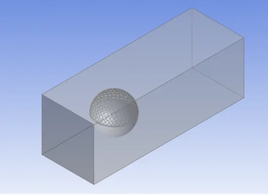
• Import the given geometry.

Meshing and Named Selection:

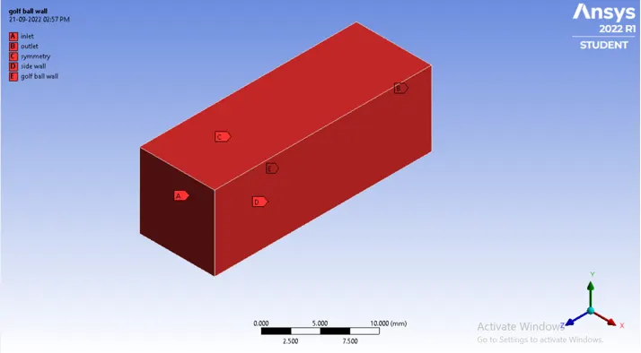
• Name selection is important for ansys to know where the flow must enter and helps in seggregating and assigning the boundary condition easily.
• Named selection for the given geometry is given below:

• Mesh details are provided below:

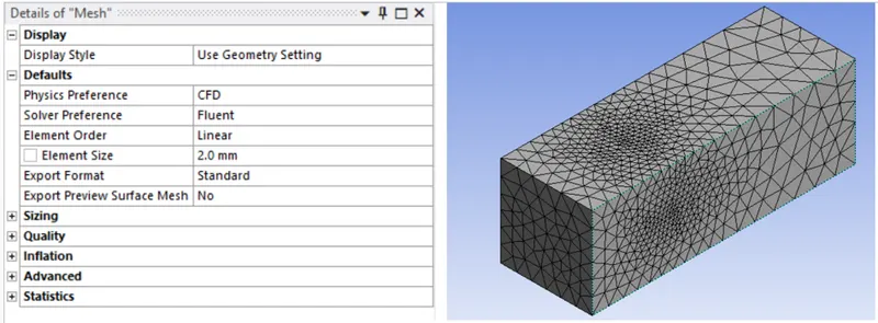
• The mesh can be refined more using different techniques but limits due to student version.

Setting up the physics:

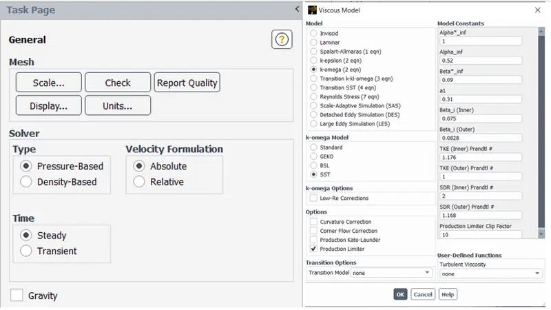
• Pressure based solver is chosen as the Mach number is less than 0.3.
• Density is considered constant.
• Turbulence Model chosen is k-omega SST model.

• Inlet Boundary condition = 60m/s.

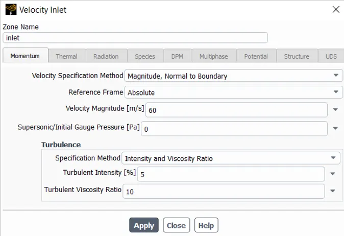
• Outlet as pressure outlet.
• Next step is to standard initialize the domain with 'compute from' as inlet.
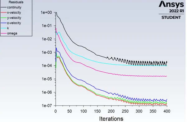
• Run it for 300 iteration.
• To be sure whether the solution has converged or not, generate a mass flow rate report before running the solution.

==============================================================================

Results:

• Residuals Plot:

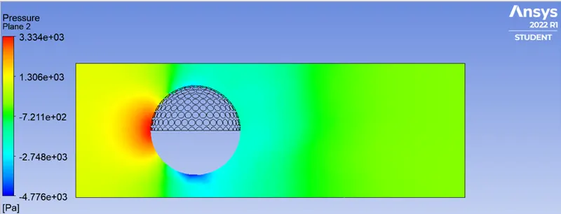
• Pressure Contour:

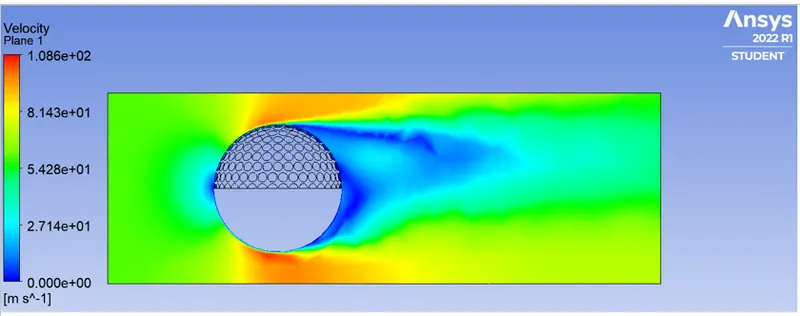
• Velocity Contour:

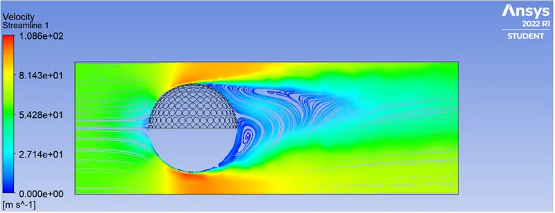
• Streamlines:

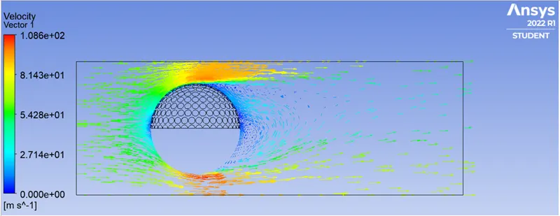
• Velocity Vector:

• Separation Point:

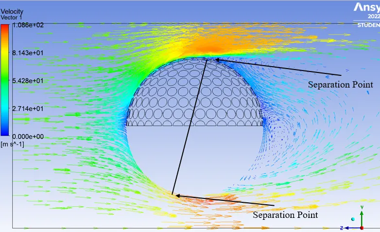
• The flow sticks to the dimple surface and separates early incase of smooth surface.
• Due to high velocity, some part of the flow below the surface tries to move with the free stream flow and some of it recirculates due to low pressure at the rear end of the ball.
• The direction of the ball will be in downward direction clockwise.

==============================================================================