Week 2 - Flow over a Cylinder.
Aim: To simulate flow over cylinder for different cases.
PART 1:
- Simulate the flow with the steady and unsteady case and calculate the Strouhal Number for Re= 100.
PART 2:
- Calculate the coefficient of drag and lift over a cylinder by setting the Reynolds number to 10,100,1000,10000 & 100000. (Run with steady solver)
- Discuss the effect of Reynolds number on the coefficient of drag. [ Results should be validated with any standard literature and error should be within 5 %].
Expected Results:
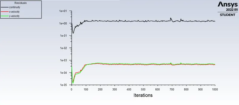
- In both approaches, show that the flow has converged. That is, what quantities or plots need to be looked at to determine that the flow has converged?
- Plots of the coefficient of drag and lift.
- Plots to show vortex shedding behind the cylinder.
- Mention the referred material (Reference Paper or Fluid Mechanics Textbook) at the end of the challenge submission page.
==============================================================================
Understanding the concept of Karman vortex street:
- In fluid dynamics, a Kármán vortex street (or a von Kármán vortex street) is a repeating pattern of swirling vorrtices, caused by a process known as vortex shedding, which is responsible for the unsteady seperation of flow of a fluid around blunt bodies.
- In this flow, vortices are created at the back of the body and detach periodically from either side of the body forming a Von Karman vortex street.
- The fluid flow past the object creates alternating low-pressure vortices on the downstream side of the object. The object will tend to move toward the low-pressure zone.
- Vortex shedding takes place at certain velocity value, usually correlated with the term 'Reynolds Number'.
- Reynolds number is the ratio of inertial forces to viscous forces and is given by formula:
`Re = (U_(infty*rho*L_(c)))/(mu)`
Re = Reynolds Number (non-dimentional number)
`U_(infty)` = Free stream velocity
`rho` = Density
`L_(c)` = Charateristic length
`mu` = Dynamic Viscosity
- Downside of the vortex shedding is, if flow over any structure sheds vortex at resonance frequency of structure, then there are high chances that it may damage the structure. Common examples are tall buildings, bridges, car antenna etc.
==============================================================================
FLOW-CHART:
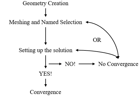
Explanation of flowchart:
- Create Geometry.
- Generate appropriate mesh.
- Set up the physics/solution.
- If it reaches convergence, the results are fine (varies from problem to problem).
- If it does not reach convergence, either you need to refine the mesh or make some changes in the solution setup.
==============================================================================
Parameter that are same for all the cases:
- Geometry
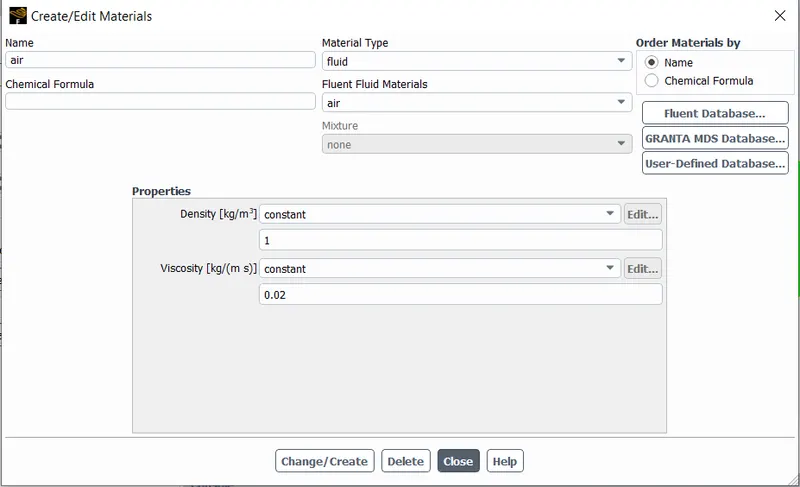
- Density = 1
- Viscosity = 0.02
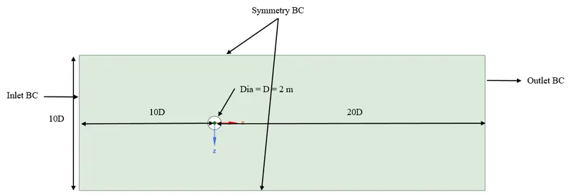
Geometry:
==============================================================================
GEOMETRY AND MESH IS SAME FOR ALL THE CASES.
- Step 1 is geometry creation.
- Step 2 is Meshing. By using method sizing and assigning triangle mesh with inflation layer near the cylinder will help capture better flow results.
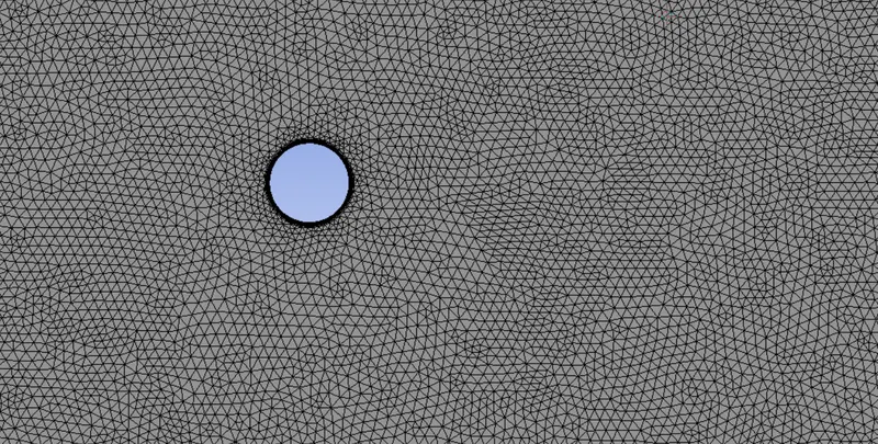
- You need to refine the mesh until you don't get the desired results (one of the options).
==============================================================================
PART 1 AND 2 PROCEDURE:
- Make sure inside viscous tab, laminar is selected. (after selecting physics)
- For material properties, select create material and change the density to 1 and dynamic viscocity to 0.02. (same for all cases).
- Select Boundaries tab and assign the required boundary condition. For inlet provide the inlet velocity, for outlet provide pressure-outlet, for cylinder assign wall and for top and bottom assign symmetry boundary condition.
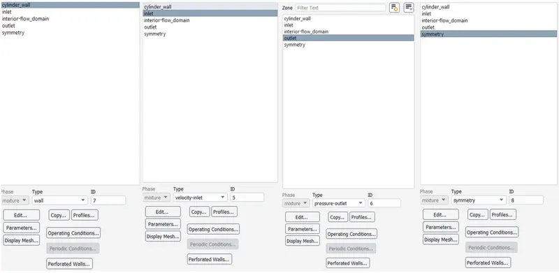
Note: Value of velocity inlet will change with respect to reynolds number. (Formula for which is provided above).
- Before starting to solve the problem we will need to place some point after the cylinder (downstream) for capturing vortex shedding phenomena.
- Switch over to results tab, and select create placed near left top corner. Select point and provide the dimensions as required and name it monitor-point or what ever you like.
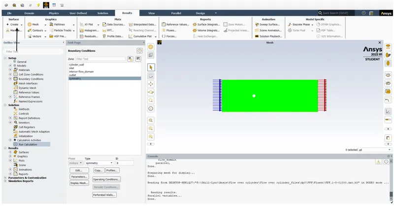
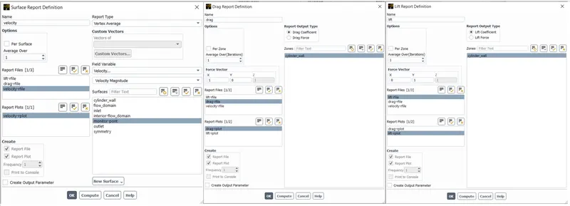
- Switch again to solutions tab and prepare few definition reports. Select surface report and then select vertex average. Then select velocity from the drop down menu and do not forget to select monito-point (your name selection).
- Follow the same procedure for drag and lift report definition.
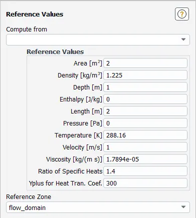
- Navigte to reference values (find it near the outline view). For Area assign value as 2 and for length assign value of 2. This calculated as Area = diameter*depth (2D, depth = 1) and length = diameter (for circle/cylinder).
- Before initializing the solution, make sure SIMPLE scheme is selected.
- Initialize the solution.
- After initializing, create contour plot inorder to create animation.
- Provide number of iteration and click on calculate. If initial number of iteration are not sufficient to capture the physics, then increase the number of iterations and remove limit to residual. (Uncheck convergence box for all residual parameters).
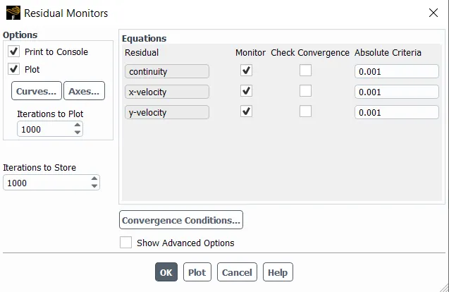
- NOTE: The procedure is same for all the cases. The only thing that is going to change is the inlet velocity by consdering different Reynolds number.
==============================================================================
RESULTS AND DISCUSSION:
- PART 1: Steady and Transient simulation for Re = 100.
STEADY STATE:
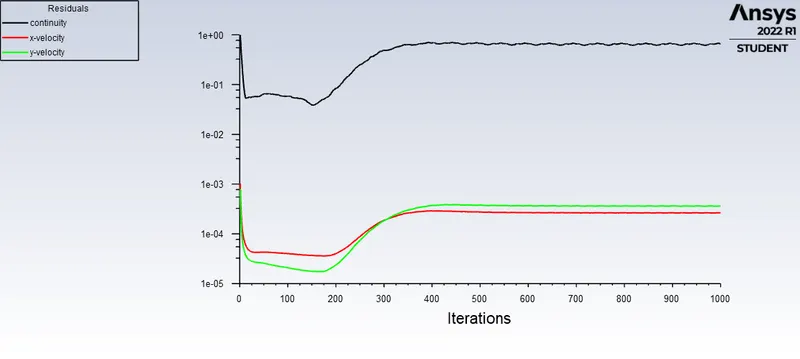
- Residual Graph:
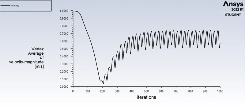
- Vertex average of velocity:
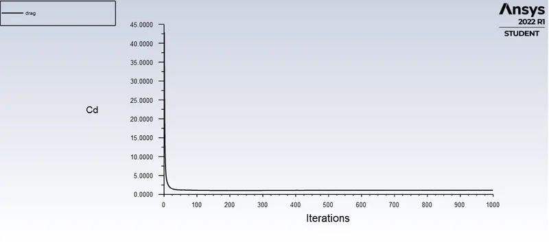
- Drag Report:
- Lift Report:
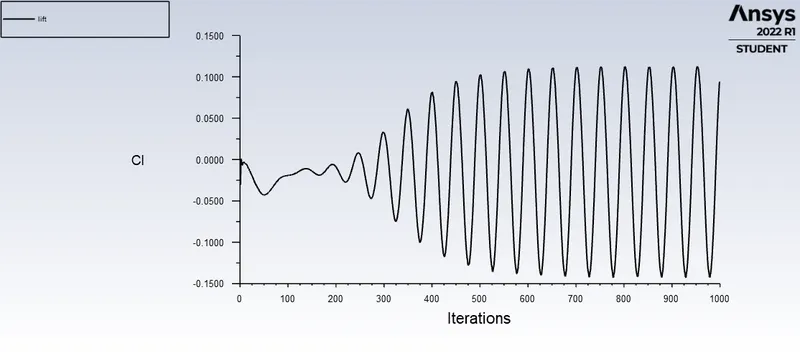
TRANSIENT:
- Residual Graph:
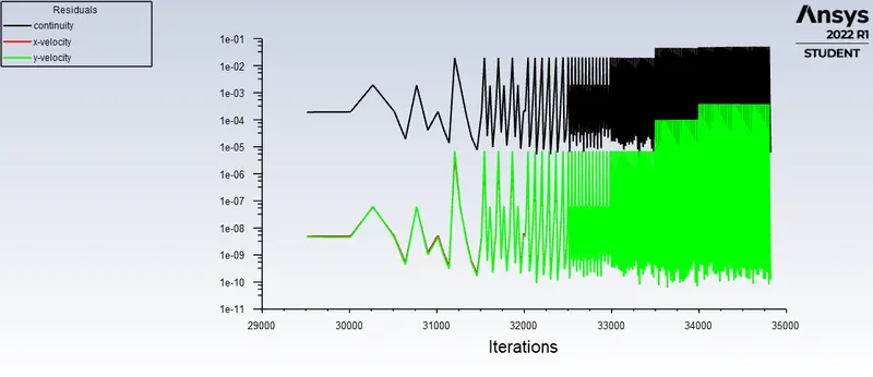
- Vertex average of velocity:
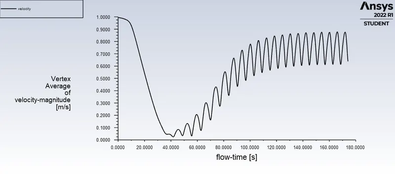
- Drag Report:
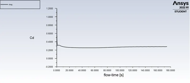
- Lift Report:
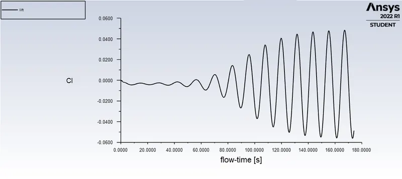
- Strouhal Number:
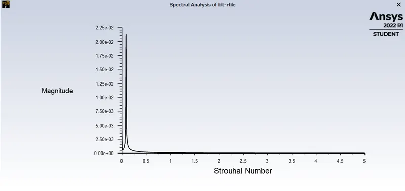
- Velocity Contour:
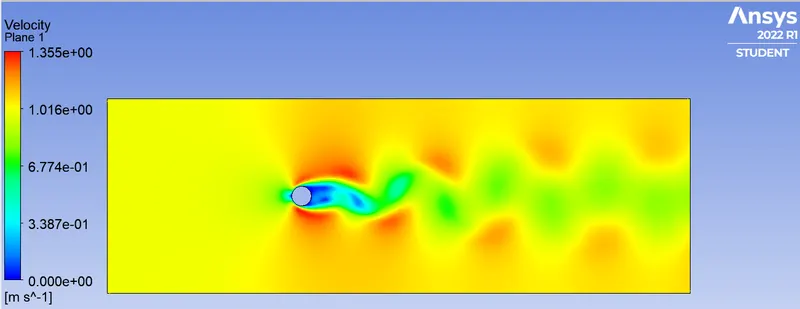
==============================================================================
PART 2: Q1. FOR Re = 10, 100, 1000, 10000, 100000.
1) Re = 10 V= 0.1 m/s
- Residual Graph:
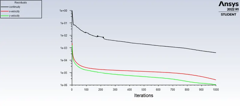
- Vertex average of velocity:
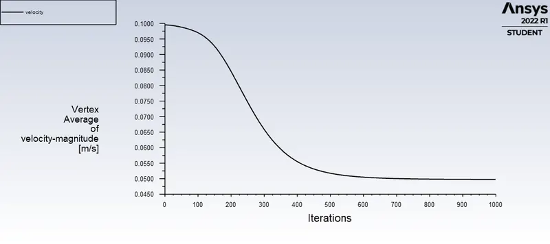
- Drag Report:
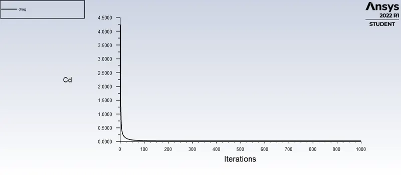
- Lift Report:
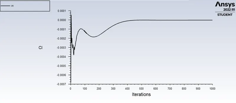
- Velocity Contour:
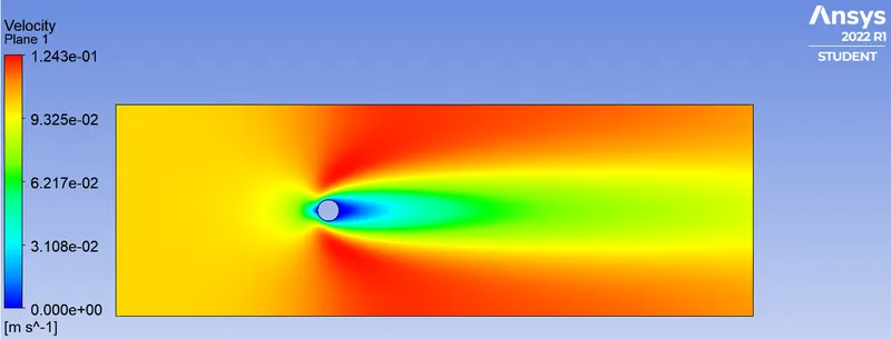
==============================================================================
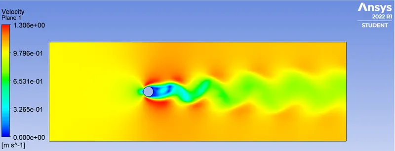
2) Re = 100 V = 1m/s
- Residual Graph:
- Vertex average of velocity:
- Drag Report:
- Lift Report:
- Velocity Contour:
==============================================================================
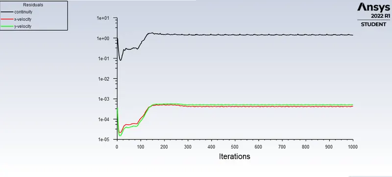
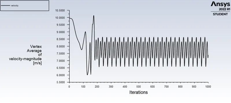
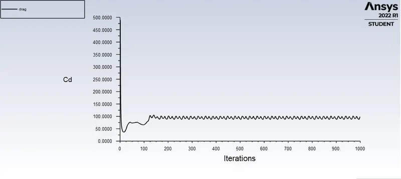
3) Re = 1000 V= 10m/s
- Residual Graph:
- Vertex average of velocity:
- Drag Report:
- Lift Report:
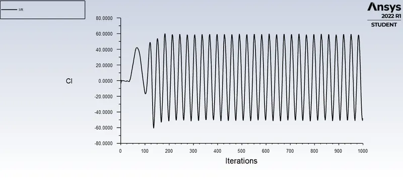
- Velocity Contour:
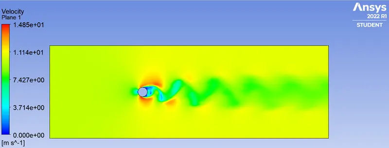
==============================================================================
4) Re = 10,000 V= 100m/s
- Residual Graph:
- Vertex average of velocity:
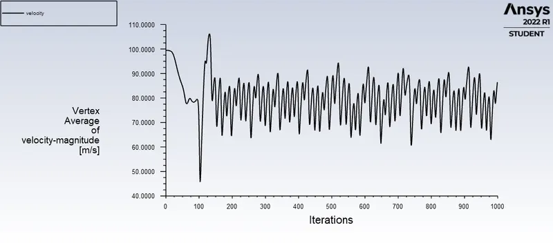
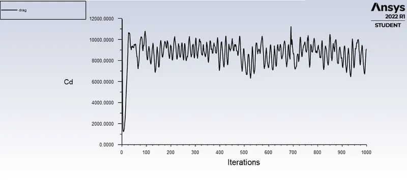
- Drag Report:
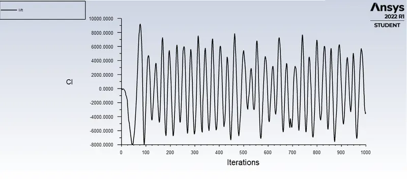
- Lift Report:
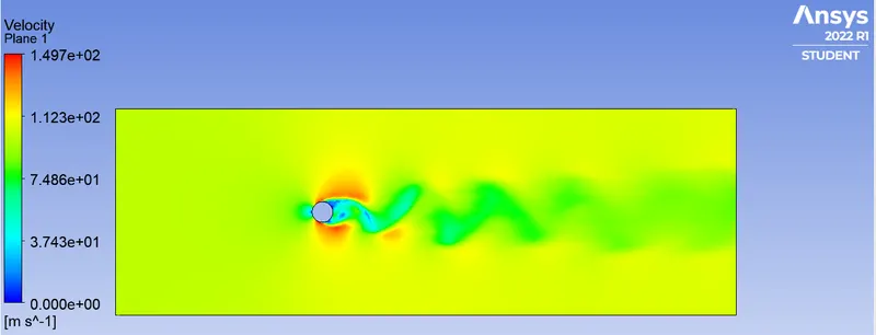
- Velocity Contour:
==============================================================================
5) Re = 1,00,000 V = 1000m/s
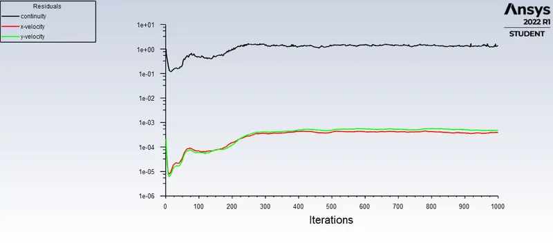
- Residual Graph:
- Vertex average of velocity:
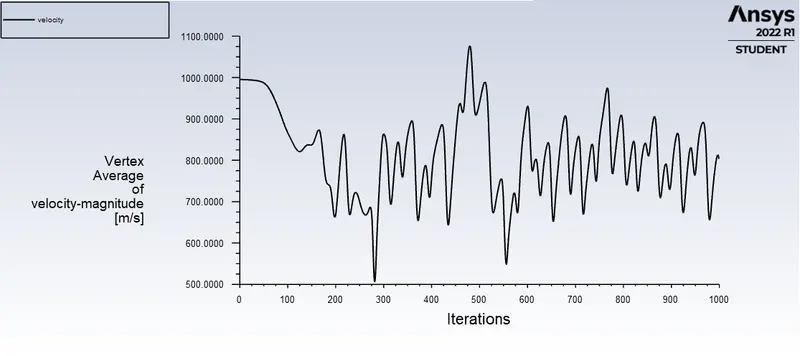
- Drag Report:
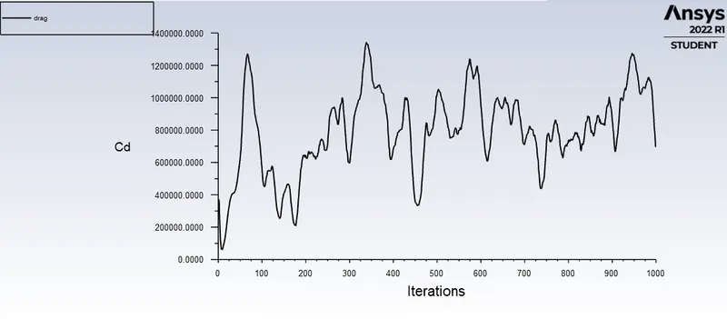
- Lift Report:
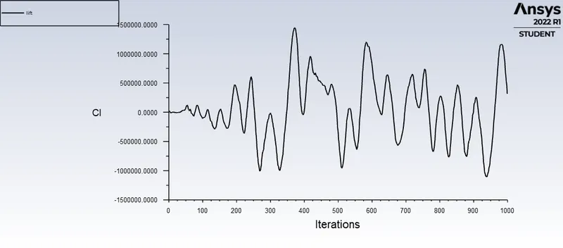
- Velocity Contour:
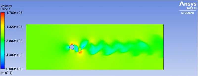
How to understand if it has reached convergence?
Ans: If the solution pattern repeats itself after certain number of iterations, then one can consider it has converged. Also check for the residual values. For example look at the vortex average velocity graph, it repeats itself periodically.
=============================================================================
DISCUSSION:
1) The vortex shedding appears very early (in terms of iteration) for high reynolds number.
2) As you increase the velocity by increasing the Reynolds Number, the solution becomes unstable and one has to tweak the relaxation factor for solution stability.
3) For high velocity the values of coefficient of drag and lift are very high.
4) For Reynolds Number higher than 10,000 it requires much more iterations to stabalise when compared to other values of Reynolds Number.
5) For low Re values it takes time to develop the wake behind the cylinder when simulating transient behaviour of flow over cylinder.
6) Vortex streaching can be seen properly when Re values are low.
7) Validation: The results do not (5%) match with the research paper. Possible reasons could be:
- Geometry.
- Density and viscosity of fluid.
- Domain.
- Solver type (Scheme type)
The only thing that matches with the paper is the physics is captured properly for lift coefficient.
| Vertex avg of velocity (m/s) | Drag | Lift | |
| Re =10 | 0.0497 | 0.0271 | -2.847e-6 |
| Re =100 | 0.5949 | 1.1028 | 0.1016 |
| Re =1000 | 7.6409 | 100.2387 | -41 |
| Re =10,000 | 87.986 | 9086.6773 | -2874.9486 |
| Re =1,00,000 | 791.2380 | 674064.54 | 290768.75 |
| Re = 100 (Transient) | 0.6381 | 0.2832 | -0.04865 |