Week 11- Broadband Noise modelling over Ahmed body

Aim: To understand what is sound and how it is generated due to intricate flows around a given body inside a domain.

Take away: By the end of this article one will be able to comprehend,

1. What is sound and how it is generated.

2. What are the models at disposal for calculating the source of noise.

3. Simulate flow around Ahmed body.

4. Plot graphs and contours required for assisment.

==============================================================================

What is Sound?

• In physics, sound is a vibration that propagates as an acoustic wave, through a transmission medium such as a gas, liquid or solid.
• In human physiology and psychology, sound is the reception of such waves and their perception by the brain.
• Only acoustic waves that have frequencies lying between about 20 Hz and 20 kHz, the audio frequency range, elicit an auditory percept in humans.
• In air at atmospheric pressure, these represent sound waves with wavelengths of 17 meters (56 ft) to 1.7 centimeters (0.67 in).
• Sound waves above 20 kHz are known as ultrasound and are not audible to humans. Sound waves below 20 Hz are known as infrasound. Different animal species have varying hearing ranges.

What is Acoustics?

• Acoustics is the interdisciplinary science that deals with the study of mechanical waves in gasses, liquids, and solids including vibration, sound, ultrasound, and infrasound.

Reference: Link

==============================================================================

Numerical Models for Acoustic calculation:

Acoustic problems can be solved numerically via three methods:

1. Direct Method

2. Integral Method by Ffowcs Williams and Hawking

3. Method based on wave equation

4. Broadband Noise Modelling

Direct Method:

• In this method, both generation and propagation of sound waves are directly computed by solving the appropriate fluid dynamics equations.
• Prediction of sound waves always requires time-accurate solutions to the governing equations. Furthermore, in most practical applications of the direct method, one has to employ governing equations that are capable of modeling viscous and turbulence effects, such as unsteady Navier-Stokes equations (that is, DNS), RANS equations, and filtered equations used in SAS / DES / SDES / SBES and LES.
• The direct method is therefore computationally difficult and expensive inasmuch as it requires highly accurate numerics, very fine computational meshes all the way to receivers, and acoustically non-reflecting boundary conditions.
• The computational cost becomes prohibitive when sound is to be predicted in the far field (for example, hundreds of chord-lengths in the case of an airfoil).
• The direct method becomes feasible when receivers are in the near field (for example, cabin noise).
• In many such situations involving near-field sound, sounds (or pseudo-sounds for that matter) are predominantly due to local hydrodynamic pressure, which can be predicted with a reasonable cost and accuracy.
• Since sound propagation is directly resolved in this method, one normally needs to solve the compressible form of the governing equations (for example, compressible RANS equations, compressible form of filtered equations for LES).
• Only in situations where the flow is low and subsonic, and the receivers in the near field consist primarily of local hydrodynamic pressure fluctuations (that is, pseudo sound), can incompressible flow formulations be used.
• However, this incompressible treatment will not permit you to simulate resonance and feedback phenomena.

Integral Method by Ffowcs Williams and Hawkings:

• For predictions of mid- to far-field noise, the methods based on Lighthill’s acoustic analogy offer viable alternatives to the direct method.
• In this approach, the near-field flow obtained from appropriate governing equations such as unsteady RANS equations, SAS / DES / SDES / SBES, or LES are used to predict the sound with the aid of analytically derived integral solutions to wave equations.
• The acoustic analogy essentially decouples the propagation of sound from its generation, enabling one to separate the flow solution process from the acoustics analysis.
• The FW-H formulation adopts the most general form of Lighthill’s acoustic analogy, and is capable of predicting sound generated by equivalent acoustic sources.
• Ansys Fluent adopts a time domain integral formulation wherein time histories of sound pressure, or acoustic signals, at prescribed receiver locations are directly computed by evaluating corresponding surface integrals.
• One important limitation of the integral FW-H formulation is that it is applicable only to predicting the propagation of sound toward free space.
• Thus, while the model can be legitimately used to predict far-field noise due to external aerodynamic flows, such as the flows around ground vehicles and aircraft, it cannot be used for predicting the noise propagation inside ducts or wall-enclosed space.

Method based on Wave Equation:

In this hybrid simulation method, which is intended to simulate aeroacoustics of low Mach number flows, the incompressible flow model is used for the calculation of sound sources, while the differential wave equation is used to calculate the propagation of sound generated by these sources.

The acoustics wave equation implemented in Ansys Fluent is derived from the acoustics perturbation equations by Ewert and Schroeder under the assumption of constant density flow.

The main advantages of this model are:

• Extended applicability compared to the Ffowcs Williams and Hawking integral solver, which can be used only to model the sound propagation in open space (see The Ffowcs Williams and Hawkings Model.
• Simple and convenient workflow of hybrid aeroacoustics simulations, without any data exchange between different software components via disk files, and without the interpolation of sound sources on a different mesh.
• A transient co-simulation of fluid flow and noise propagation using the same domain and mesh has been chosen for the current implementation.
• The method includes the Kirchhoff integral tool to propagate the wave equation solution to the remote receivers in open space.

Broadband Noise Source Model:

• In many practical applications involving turbulent flows, noise does not have any distinct tones, and the sound energy is continuously distributed over a broad range of frequencies.
• In those situations involving broadband noise, statistical turbulence quantities readily computable from RANS equations can be utilized, in conjunction with semi-empirical correlations and Lighthill’s acoustic analogy, to shed some light on the source of broadband noise.

Reference: Ansys Theory Guide

==============================================================================

What is Ahmed Body?

• Ahmed body is the the simplified form of a car. Its simplified body helps in carrying out experiments with scale down version.
• It helps in capturing same physics which might be similar or close to a detailed car model.
• It is also known as bluf body.
• Parametric study becomes much more easier by making geometrical changes to the body.

==============================================================================

Simulation Procedure:

Geometry:

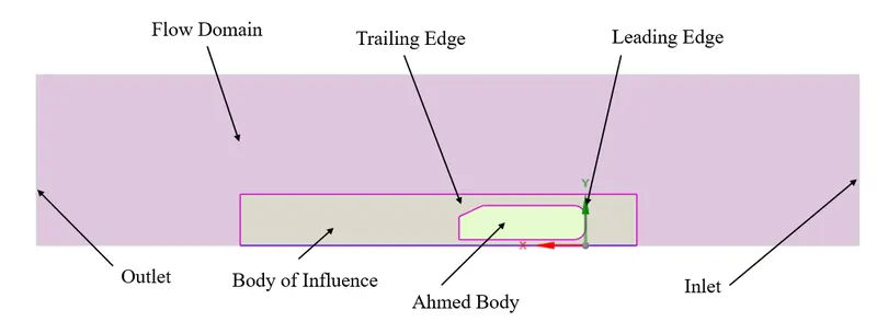
Meshing Strategy:

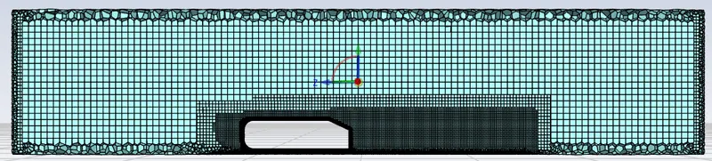
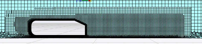
• In this challange I have used Ansys Fluent Water Tight Meshing.
• It is also know as Ansys Mosiac Meshing.
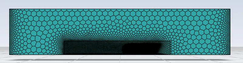
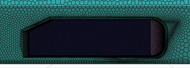
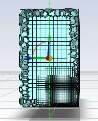
• Rather than creating tetrahedral mesh, it creates Poly-Hexcore mesh.
• Where ever it finds volume with out curvature, it creates hex mesh.
• On the surface and near the transition from poly to hex region, it creates Polygonal mesh.
• It is efficient and requires less memory and mesh elements to capture same physics phenomena compared to other mesh element types.
• The heighest quality results are obtained via this mesh after hexahedral mesh type.

Step 1: Import geometry

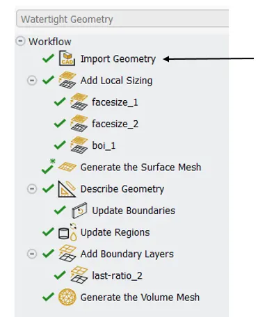
Step 2: Add local refinement

• Specfiy local target mesh to a specific face, body or use body of influence to create fine mesh around the region of interest.
• It is similar to what we do in conventional mesh method.

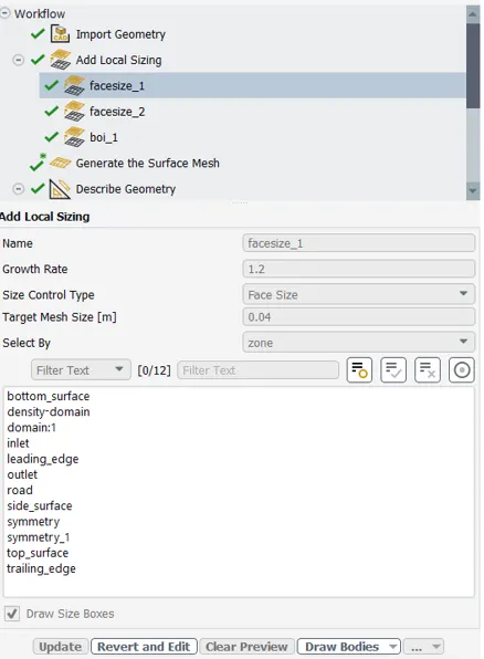
• Assign the target mesh size to the selected face or body.
• Similarly refine accordingly so as to capture the geometry properly.

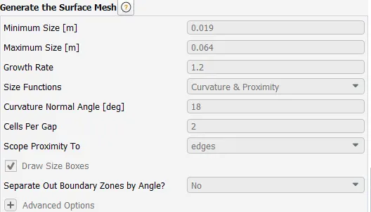
Step 3: create Surface Mesh

• Create a surface mesh according to your degree of refinement.
• I am restricted with mesh elements upto 512K.
• Specify min and max value for the mesh size.

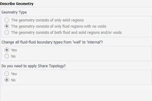
Step 4: Describe the geometry

• It will ask you few questions regarding the geometry.
• For example, Does the goemetry have fluid regions, solid regions, or both solid and fluid.
• Convert all the fluid from wall to internal - yes
• No to share topology if already done in spaceclaim.
• Choose according to flow physics you want to capture.

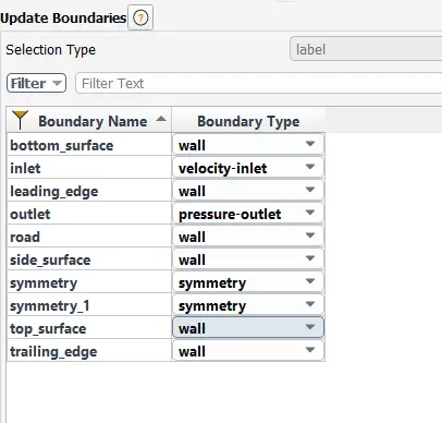
Step 5: Update boundaries

• Assign the right boundary condition.
• Not to worry if assigned it wrong, one can change in fluent solver.

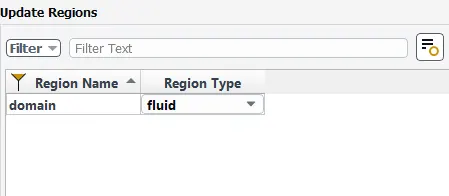
Step 6: Update regions

• Specify which solid body is "Solid" or "Fluid".
• In this case we only have 1 fluid region.

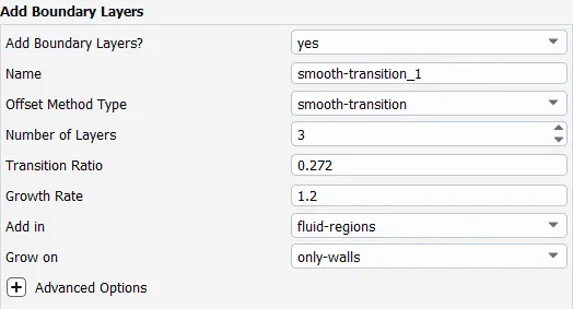
Step 7: Add Boundary Layers

• It is very crucial step to add boundary layer to capture the boundary layer phenomena close to surface properly.

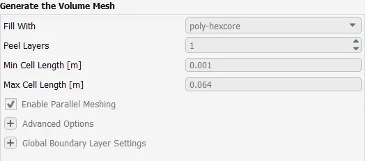
Step 8: Volume Mesh

• Final step is to create a volume mesh.
• Select Poly-Hecore type.
• One cannot change the min and max element size values. It is to capture the geometry properly.

Mesh:

==============================================================================

Simulation Setup:

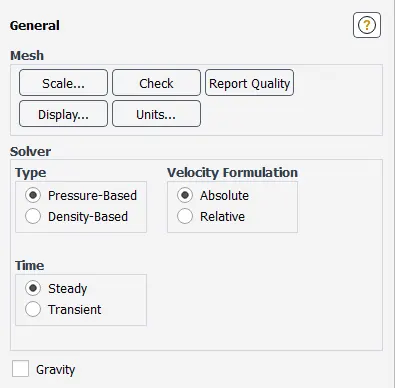
General:

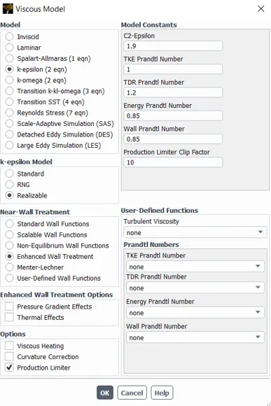
Viscous Model:

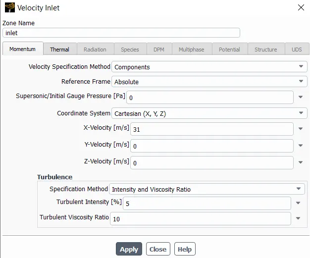
Boundary Condition:

• Velocity = 31m/s
• Outlet = pressure outlet

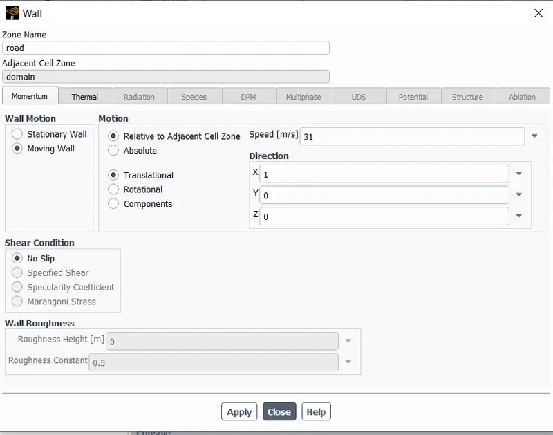
• Road is a moving wall.

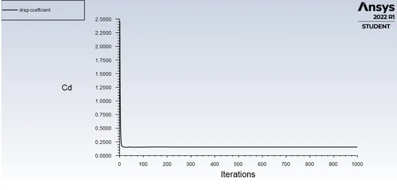
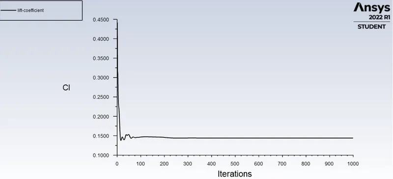
• Plot the results for Cd and Cl.
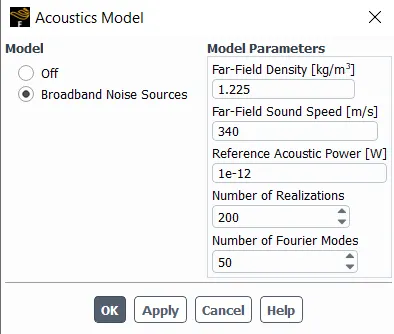
• Run the simulation wih the acoustic model swithced off.
• Once the simulation has converged and is satisfactory, turn on the acousticc model.

==============================================================================

Results:

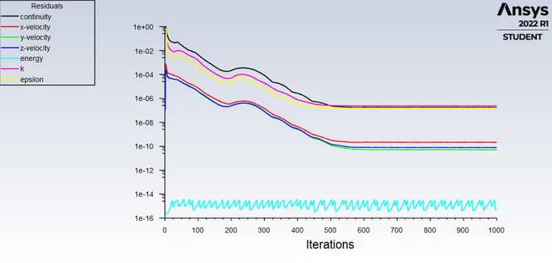
• Residual:

• Coefficient of Drag:

• Coefficient of Lift:

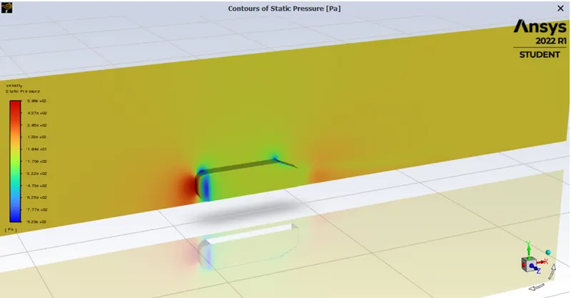
• Static Pressure:

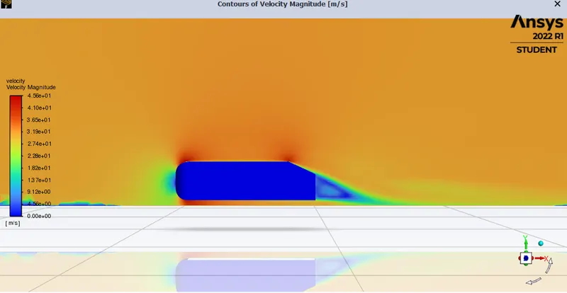
• Velocity Magnitude:

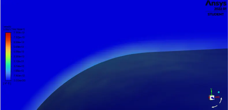
• Lilly's Total Noise Source:

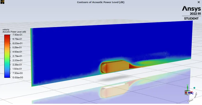
• Acoustic Power Level (dB):

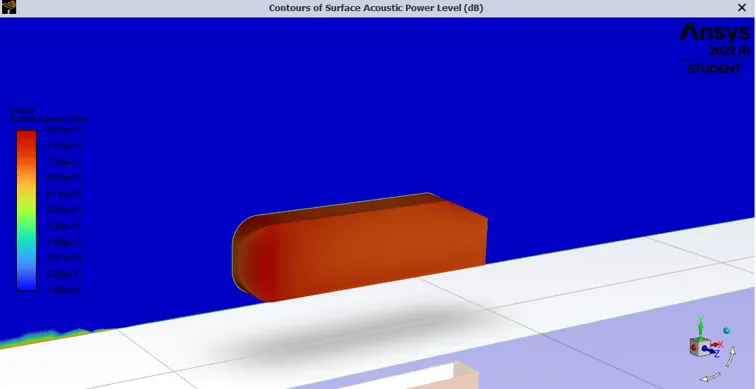
• Surface Acoustic Power Level (dB):

==============================================================================

Conclusion:

• Surface Acoustic Power Level is under the threshold limit. With mesh refinement one might get a better result.
• Overall, the solution is converged, but the results will change with respect to mesh size. Grid Independece Test is must.
• One might be familiar with the concept of Acoustic model.