Week 7 - Simulation of a 1D Super-sonic nozzle flow simulation using Macormack Method

Aim: The aim of this project is to understand the concept of CFD and apply it to a physical problem, get a hands on experience of coding such a problem statement.

Problem Statement: In this particular project, we have performed 1D simulation of subsonic-supersonic isentropic nozzle flow using Macormack technique.

Objective: After completion of project, we will be able to structure code for the given problem statement and have it observed with the help of plots. Understand the theoretical aspect of the problem statement and proceed with the simulation.

Understanding the problem statement:

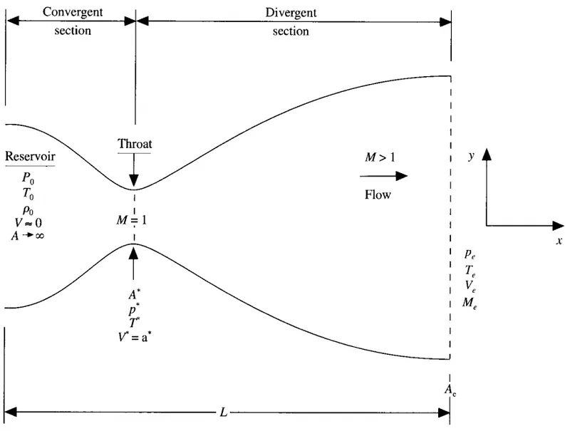
The above figure is of convergent divergent nozzle.

• Flow through the nozzle comes from reservoir where the pressere and tepmerature are Po and To respectively.
• It is assumed (theoretically) that the cros-sectional area of the reservoir is very large hence the velocity at the inlet is close to 0.
• Pe, Te, Ve, Me are the pressure, temperature, velocity, Mach Number at the outlet or the exit of the nozzle.
• We have assumed that flow properties are varying only in x direction.

==============================================================================

Governing Equations for Quasi 1D, steady, isentropic flow for continuity, momentum and energy equations are given below:

• Continuity:

`\begin{equation} \rho_{1} V_{1} A_{1}=\rho_{2} A_{2} V_{2} \end{equation}`

• Momentum:

`\begin{equation} p_{1} A_{1}+\rho_{1} V_{1}^{2} A_{1}+\int_{A_{1}}^{A_{2}} p d A=p_{2} A_{2}+\rho_{2} V_{2}^{2} A_{2} \end{equation}`

• Energy:

`\begin{equation} h_{1}+\frac{V_{1}^{2}}{2}=h_{2}+\frac{V_{2}^{2}}{2} \end{equation}`

==============================================================================

Setup:

The whole setup is divided into 3 parts:

1. Governing Equations for Quasi 1D subsonic-supersonic isentropic nozzle flow.
2. Numerical descritization.
3. Other important parameters such as time calculation, boundary conditions etc.

Governing Equations:

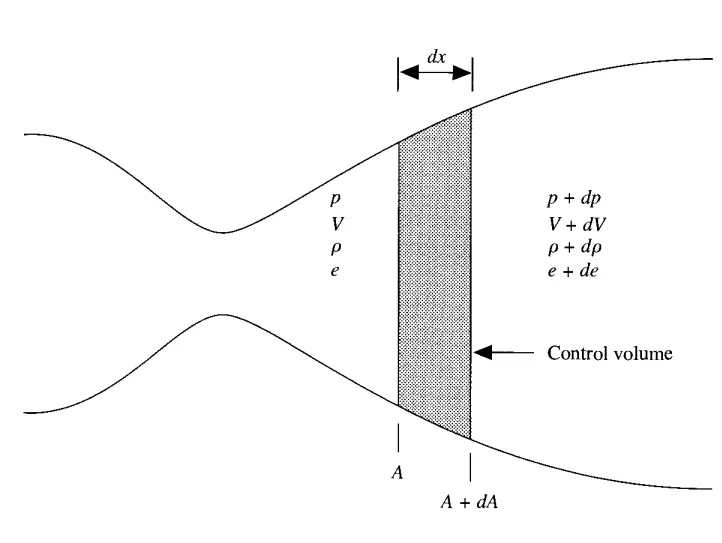
• The shaded region is the considered infinitesimal element with dx as length.

Starting with the Integral form of equation for CONTINUITY EQUATION:

`\begin{equation} \frac{\partial}{\partial t} \iiint_{\mathscr{V}} \rho d \mathscr{V}+\iint_{S} \rho \mathbf{V} \cdot \mathbf{d S}=0 \end{equation}`

On the LHS we have the volume integral and the surface integral equating to 0.

The volume integral can be written as,

`\begin{equation} \frac{\partial}{\partial t} \iiint \rho d \mathscr{V}=\frac{\partial}{\partial t}(\rho A d x) \end{equation}`

And the surface integral can be written as,

`\begin{equation} \iint_{S} \rho \mathbf{V} \cdot \mathbf{d S}=-\rho V A+(\rho+d \rho)(V+d V)(A+d A) \end{equation}`

Simplifying the surface integral,

`\begin{equation} \begin{aligned} \iint \rho \mathbf{V} \cdot \mathbf{d S}=&-\rho V A+\rho V A+\rho V d A+\rho A d V+\rho d V d A \\ &+A V d \rho+V d A d \rho+A d V d \rho+d \rho d V d A \end{aligned} \end{equation}`

All the terms involving theproducts of differential can be considered 0, and equation of surface integral becomes,

`\begin{equation} \iint_{S} \rho \mathbf{V} \cdot \mathbf{d S}=\rho V d A+\rho A d V+A V d \rho=d(\rho A V) \end{equation}`

Therefore,

`\begin{equation} \frac{\partial}{\partial t}(\rho A d x)+d(\rho A V)=0 \end{equation}`

Finally dividing throught by dx and as dx tends to zero,

`\begin{equation} \frac{\partial(\rho A)}{\partial t}+\frac{\partial(\rho A V)}{\partial x}=0 \end{equation}`

The above equation represents the continuity equation for quasi 1D subsonic supersonic isentropic unsteady nozzle flow.

Starting with the X-COMPONENT OF MOMENTUM EQUATION:

`\begin{equation} \frac{\partial}{\partial t} \iiint_{\mathscr{V}}(\rho u) d \mathscr{V}+\iint_{S}(\rho u \mathbf{V}) \cdot \mathbf{d S}=-\iint_{S}(p d S)_{x} \end{equation}`

Intergrals on the LHS are evaluated in similar manner as above,

Volume Integral,

`\begin{equation} \frac{\partial}{\partial t} \iiint_{\mathscr{V}}(\rho u) d \mathscr{V}=\frac{\partial}{\partial t}(\rho V A d x) \end{equation}`

Surface Integral,

`\begin{equation} \iint_{S}(\rho u \mathbf{V}) \cdot \mathbf{d S}=-\rho V^{2} A+(\rho+d \rho)(V+d V)^{2}(A+d A) \end{equation}`

The RHS is expressed as,

`\begin{equation} \iint(p d S)_{x}=-p A+(p+d p)(A+d A)-2 p\left(\frac{d A}{2}\right) \end{equation}`

After getting all the equations we can write it as,

`\begin{equation} \begin{aligned} \frac{\partial}{\partial t}(\rho V A d x)-\rho V^{2} A+(\rho+d \rho)(V+&d V)^{2}(A+d A) \\ &=p A-(p+d p)(A+d A)+p d A \end{aligned} \end{equation}`

cancelling like terms, product differentials and dx tends to 0, we have,

`\begin{equation} \frac{\partial}{\partial t}(\rho V A d x)+d\left(\rho V^{2} A\right)=-A d p \end{equation}`

As dx tends to 0,

`\begin{equation} \frac{\partial(\rho V A)}{\partial t}+\frac{\partial\left(\rho V^{2} A\right)}{\partial x}=-A \frac{\partial p}{\partial x} \end{equation}`

The above equation is in the conservation form.

To convert it into non conservation form we must multiply the above equation with V.

Therefore,

`\begin{equation} V \frac{\partial(\rho A)}{\partial t}+V \frac{\partial(\rho V A)}{\partial x}=0 \end{equation}`

Now subtracting the above equation and the conservative form we get

`\begin{equation} \frac{\partial(\rho V A)}{\partial t}-V \frac{\partial(\rho A)}{\partial t}+\frac{\partial\left(\rho V^{2} A\right)}{\partial x}-V \frac{\partial(\rho V A)}{\partial x}=-A \frac{\partial p}{\partial x} \end{equation}`

Expanding derivatives on LHS and canceling like terms,we get,

`\begin{equation} \rho A \frac{\partial V}{\partial t}+\rho A V \frac{\partial V}{\partial x}=-A \frac{\partial p}{\partial x} \end{equation}`

Divide throught by A,

`\begin{equation} \rho \frac{\partial V}{\partial t}+\rho V \frac{\partial V}{\partial x}=-\frac{\partial p}{\partial x} \end{equation}`

The above equation represents the conservation form of equation of X-component of Momentum Equation.

Finally lets consider the ENERGY EQUATION:

`\begin{equation} \frac{\partial}{\partial t} \iiint_{\mathscr{Y}} \rho\left(e+\frac{V^{2}}{2}\right) d \mathscr{V} \cdot+\iint_{S} \rho\left(e+\frac{V^{2}}{2}\right) \mathbf{V} \cdot \mathbf{d S}=-\iint_{S}(p \mathbf{V}) \cdot \mathbf{d S} \end{equation}`

On further simplification,

`\begin{equation} \begin{aligned} \frac{\partial}{\partial t}\left[\rho\left(e+\frac{V^{2}}{2}\right) A d x\right]-\rho\left(e+\frac{V^{2}}{2}\right) V A \\ &+(\rho+d \rho)\left[e+d e+\frac{(V+d V)^{2}}{2}\right](V+d V)(A+d A) \\ =&-\left[-p V A+(p+d p)(V+d V)(A+d A)-2\left(p V \frac{d A}{2}\right)\right] \end{aligned} \end{equation}`

Neglecting prodct of differential and canceling like terms we get,

`\begin{equation} \frac{\partial}{\partial t}\left[\rho\left(e+\frac{V^{2}}{2}\right) A d x\right]+d(\rho e V A)+\frac{d\left(\rho V^{3} A\right)}{2}=-d(p A V) \end{equation}`

or,

`\begin{equation} \frac{\partial}{\partial t}\left[\rho\left(e+\frac{V^{2}}{2}\right) A d x\right]+d\left[\rho\left(e+\frac{V^{2}}{2}\right) V A\right]=-d(p A V) \end{equation}`

Dividing throught by dx and taking the limit dx tends to 0,

`\begin{equation} \frac{\partial\left[\rho\left(e+V^{2} / 2\right) A\right]}{\partial t}+\frac{\partial\left[\rho\left(e+V^{2} / 2\right) V A\right]}{\partial x}=-\frac{\partial(p A V)}{\partial x} \end{equation}`

The above equation is the conservation form of unsteady, quasi 1D flow, the non-conservation form can be achieved by multiplying the above equation by V. Therefore we get,

`\begin{equation} \frac{\partial\left[\rho\left(V^{2} / 2\right) A\right]}{\partial t}+\frac{\partial\left[\rho\left(V^{3} / 2\right) A\right]}{\partial x}=-A V \frac{\partial p}{\partial x} \end{equation}`

Subtracting the the above equation from the conservation form equation, we get,

`\begin{equation} \frac{\partial(\rho e A)}{\partial t}+\frac{\partial(\rho e V A)}{\partial x}=-p \frac{\partial(A V)}{\partial x} \end{equation}`

Expanding the RHS and dividing by A,

`\begin{equation} \rho \frac{\partial e}{\partial t}+\rho V \frac{\partial e}{\partial x}=-p \frac{\partial V}{\partial x}-p V \frac{\partial(\ln A)}{\partial x} \end{equation}`

This equation is in terms of internal energy and is unsteady quasi 1D flow in non conservative from. The above equation is in the form of energy because for a perfect calorically gas, the equation can be written in terms of temperature. Therefore for calorically perfect gas,

`\begin{equation} e=c_{v} T \end{equation}`

Therefore the non-conservation form of energy equation is simplified to,

`\begin{equation} \rho c_{v} \frac{\partial T}{\partial t}+\rho V c_{v} \frac{\partial T}{\partial x}=-p \frac{\partial V}{\partial x}-p V \frac{\partial(\ln A)}{\partial x} \end{equation}`

From the continuity, momentum and energy equation we come to conclusion that we have 4 unknowns and 3 equations. We can eliminate pressure as,

`\begin{equation} p=\rho R T \end{equation}`

Therefore, its derivative is given by,

`\begin{equation} \frac{\partial p}{\partial x}=R\left(\rho \frac{\partial T}{\partial x}+T \frac{\partial \rho}{\partial x}\right) \end{equation}`

Now summerizing the continuity, momentum and energy equation,

Continuity:

`\begin{equation} \frac{\partial(\rho A)}{\partial t}+\rho A \frac{\partial V}{\partial x}+\rho V \frac{\partial A}{\partial x}+V A \frac{\partial \rho}{\partial x}=0 \end{equation}`

Momentum in X-direction:

`\begin{equation} \rho \frac{\partial V}{\partial t}+\rho V \frac{\partial V}{\partial x}=-R\left(\rho \frac{\partial T}{\partial x}+T \frac{\partial \rho}{\partial x}\right) \end{equation}`

Energy:

`\begin{equation} \rho c_{v} \frac{\partial T}{\partial t}+\rho V c_{v} \frac{\partial T}{\partial x}=-\rho R T\left[\frac{\partial V}{\partial x}+V \frac{\partial(\ln A)}{\partial x}\right] \end{equation}`

Usually the CFD solutions are simulated on the basis of above given governing equation (for our problem) which gives a feeling of magnitude of real physical quantities. However for this problem the governing equations are converted into non-dimentional form and solved for the CFD simulation.

For temperature and density,

`\begin{equation} T^{\prime}=\frac{T}{T_{0}} \quad \rho^{\prime}=\frac{\rho}{\rho_{0}} \end{equation}`

For length,

`\begin{equation} x^{\prime}=\frac{x}{L} \end{equation}`

Speed of sound,

`\begin{equation} a_{0}=\sqrt{\gamma R T_{0}} \end{equation}`

For velocity,

`\begin{equation} V^{\prime}=\frac{V}{a_{0}} \end{equation}`

For time,

`\begin{equation} t^{\prime}=\frac{t}{L / a_{0}} \end{equation}`

For area,

`\begin{equation} A^{\prime}=\frac{A}{A^{*}} \end{equation}`

Please note that variables with prime denotion are the non dimentionalized variables. These are substituted in the continuity, momentum and energy equation respectively.

Continuity:

`\begin{equation} \frac{\partial \rho^{\prime}}{\partial t^{\prime}}=-\rho^{\prime} \frac{\partial V^{\prime}}{\partial x^{\prime}}-\rho^{\prime} V^{\prime} \frac{\partial\left(\ln A^{\prime}\right)}{\partial x^{\prime}}-V^{\prime} \frac{\partial \rho^{\prime}}{\partial x^{\prime}} \end{equation}`

Momentum in X- direction:

`\begin{equation} \frac{\partial V^{\prime}}{\partial t^{\prime}}=-V^{\prime} \frac{\partial V^{\prime}}{\partial x^{\prime}}-\frac{1}{\gamma}\left(\frac{\partial T^{\prime}}{\partial x^{\prime}}+\frac{T^{\prime}}{\rho^{\prime}} \frac{\partial \rho^{\prime}}{\partial x^{\prime}}\right) \end{equation}`

Energy:

`\begin{equation} \frac{\partial T^{\prime}}{\partial t^{\prime}}=-V^{\prime} \frac{\partial T^{\prime}}{\partial x^{\prime}}-(\gamma-1) T^{\prime}\left[\frac{\partial V^{\prime}}{\partial x^{\prime}}+V^{\prime} \frac{\partial\left(\ln A^{\prime}\right)}{\partial x^{\prime}}\right] \end{equation}`

==============================================================================

FINITE DIFFFERENCE EQUATION

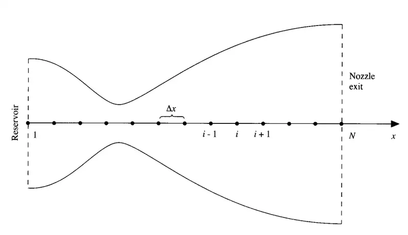
• Node number 1 is at the reservoir.
• dx is considered as the distance between the two nodes.
• The whole nozzle is divided into N number of grid points.

Predictor Step:

In this step the spatial derivatives of the governing equations are discritized with forward differencing.

Therefore, time derivative of density, velocity and temperature is calculated and is given as,

Time derivative of density,

`\begin{equation} \left(\frac{\partial \rho}{\partial t}\right)_{i}^{t}=-\rho_{i}^{t} \frac{V_{i+1}^{t}-V_{i}^{t}}{\Delta x}-\rho_{i}^{t} V_{i}^{t} \frac{\ln A_{i+1}-\ln A_{i}}{\Delta x}-V_{i}^{t} \frac{\rho_{i+1}^{t}-\rho_{i}^{t}}{\Delta x} \end{equation}`

Time derivative of velocity,

`\begin{equation} \left(\frac{\partial V}{\partial t}\right)_{i}^{t}=-V_{i}^{t} \frac{V_{i+1}^{t}-V_{i}^{t}}{\Delta x}-\frac{1}{\gamma}\left(\frac{T_{i+1}^{t}-T_{i}^{t}}{\Delta x}+\frac{T_{i}^{t}}{\rho_{i}^{t}} \frac{\rho_{i+1}^{t}-\rho_{i}^{t}}{\Delta x}\right) \end{equation}`

Time derivative of temperature,

`\begin{equation} \left(\frac{\partial T}{\partial t}\right)_{i}^{t}=-V_{i}^{t} \frac{T_{i+1}^{t}-T_{i}^{t}}{\Delta x}-(\gamma-1) T_{i}^{t}\left(\frac{V_{i+1}^{t}-V_{i}^{t}}{\Delta x}+V_{i}^{t} \frac{\ln A_{i+1}-\ln A_{i}}{\Delta x}\right) \end{equation}`

After the predictor step is performed we must update the values of density, velocity and tepmerature.

`\begin{equation} \begin{aligned} &\bar{\rho}_{i}^{t+\Delta t}=\rho_{i}^{t}+\left(\frac{\partial \rho}{\partial t}\right)_{i}^{t} \Delta t \\ &\bar{V}_{i}^{t+\Delta t}=V_{i}^{t}+\left(\frac{\partial V}{\partial t}\right)_{i}^{t} \Delta t \\ &\bar{T}_{i}^{t+\Delta t}=T_{i}^{t}+\left(\frac{\partial T}{\partial t}\right)_{i}^{t} \Delta t \end{aligned} \end{equation}`

Please note that before even starting the simulation, we have to provide the initial conditions for density, velocity and temperature. Initial conditions will be discussed in the later part of the section.

Corrector Step:

In this step we discritize the spatial derivative with rearward differencing.

Time derivative of density,

`\begin{equation} \begin{aligned} \left(\frac{\overline{\partial \rho}}{\partial t}\right)_{i}^{t+\Delta t}=&-\bar{\rho}_{i}^{t+\Delta t} \frac{\bar{V}_{i}^{t+\Delta t}-\bar{V}_{i-1}^{t+\Delta t}}{\Delta x}-\bar{\rho}_{i}^{t+\Delta t} \bar{V}_{i}^{t+\Delta t} \frac{\ln A_{i}-\ln A_{i-1}}{\Delta x} \\ &-\bar{V}_{i}^{t+\Delta t} \frac{\bar{\rho}_{i}^{t+\Delta t}-\bar{\rho}_{i-1}^{t+\Delta t}}{\Delta x} \end{aligned} \end{equation}`

Time derivative of velocity,

`\begin{equation} (\overline{\partial \bar{V}})_{i}^{t+\Delta t}=-\bar{V}_{i}^{t+\Delta t} \frac{\bar{V}_{i}^{t+\Delta t}-\bar{V}_{i-1}^{t+\Delta t}}{\Delta x}-\frac{1}{\gamma}\left(\frac{\bar{T}_{i}^{t+\Delta t}-\bar{T}_{i-1}^{t+\Delta t}}{\Delta x}+\frac{\bar{T}_{i}^{t+\Delta t}}{\bar{\rho}_{i}^{t+\Delta t}} \frac{\bar{\rho}_{i}^{t+\Delta t}-\bar{\rho}_{i-1}^{t+\Delta t}}{\Delta x}\right) \end{equation}`

Time derivative of temperature,

`\begin{equation} \begin{aligned} \left(\overline{\frac{\partial T}{\partial t}}\right)_{i}^{t+\Delta t}=&-\bar{V}_{i}^{t+\Delta t} \frac{\bar{T}_{i}^{t+\Delta t}-\bar{T}_{i-1}^{t+\Delta t}}{\Delta x}-(\gamma-1) \bar{T}_{i}^{t+\Delta t} \\ & \times\left(\frac{\bar{V}_{i}^{t+\Delta t}-\bar{V}_{i-1}^{t+\Delta t}}{\Delta x}+\bar{V}_{i}^{t+\Delta t} \frac{\ln A_{i}-\ln A_{i-1}}{\Delta x}\right) \end{aligned} \end{equation}`

Now taking the average time derivative of density, velocity and temperature

`\begin{equation} \begin{aligned} &\left(\frac{\partial \rho}{\partial t}\right)_{\mathrm{av}}=0.5[\underbrace{\left[\frac{\partial \rho}{\partial t}\right)_{i}^{t}}_{\substack{\text { From Eq. } \\(7.51)}}+\underbrace{\left(\frac{\partial \rho}{\partial t}\right)_{i}^{t+\Delta t}}_{\substack{\text { From Eq. } \\(7.57)}}]\\ &\left(\frac{\partial V}{\partial t}\right)_{\mathrm{av}}=0.5[\underbrace{\left(\frac{\partial V}{\partial t}\right)_{i}^{t}}_{\substack{\text { From Eq. } \\(7.52)}}+\underbrace{\left(\frac{\partial V}{\partial t}\right)_{i}^{t+\Delta t}}_{\substack{\text { From Eq. } \\(7.58)}}]\\ &\left(\frac{\partial T}{\partial t}\right)_{\mathrm{av}}=0.5[\underbrace{\left(\frac{\partial T}{\partial t}\right)_{i}^{t}}_{\substack{\text { From Eq. } \\(7.53)}}+\underbrace{\left(\frac{\overline{\partial T}}{\partial t}\right)_{i}^{t+\Delta t}}_{\substack{\text { From Eq. } \\(7.59)}}] \end{aligned} \end{equation}`

Now finally updating the value of our primitive variables,

`\begin{equation} \begin{aligned} \rho_{i}^{t+\Delta t} &=\rho_{i}^{t}+\left(\frac{\partial \rho}{\partial t}\right)_{\mathrm{av}} \Delta t \\ V_{i}^{t+\Delta t} &=V_{i}^{t}+\left(\frac{\partial V}{\partial t}\right)_{\mathrm{av}} \Delta t \\ T_{i}^{t+\Delta t} &=T_{i}^{t}+\left(\frac{\partial T}{\partial t}\right)_{\mathrm{av}} \Delta t \end{aligned} \end{equation}`

CALCULATION OF TIME STEP:

`\begin{equation} \Delta t=C \frac{\Delta x}{a+V} \end{equation}`

C = courant number

a = speed of sound

V = velocity of fluid/gas.

The value of dt is decided as the minimum value of dt calculated for every grid point.

`\begin{equation} \Delta t=\operatorname{minimum}\left(\Delta t_{1}^{t}, \Delta t_{2}^{t}, \ldots, \Delta t_{i}^{t}, \ldots, \Delta t_{N}^{t}\right) \end{equation}`

Equation:

At ith grid point,

`\begin{equation} (\Delta t)_{i}^{t}=C \frac{\Delta x}{a_{i}^{t}+V_{i}^{t}} \end{equation}`

At (i+1)th grid point,

`\begin{equation} (\Delta)_{i+1}^{t}=C \frac{\Delta x}{a_{i+1}^{t}+V_{i+1}^{t}} \end{equation}`

BOUNDARY CONDITIONS:

The boundary conditions are the most essential part of any CFD simulation procedure without which one cannot start the simulation or might get absurd values of the flow properties/variables.

The boundary conditions for any given problem can be decided with the help of method of characteristics. Detail explanation for the same can be found in John Anderson textbook.

We will stick to the boundary conditions for this problem.

Inflow Boundary Condition,

`\begin{equation} \text { Slope }=\frac{V_{3}-V_{2}}{\Delta x} \end{equation}`

`\begin{equation} \begin{aligned} &V_{1}=V_{2}-\frac{V_{3}-V_{2}}{\Delta x} \Delta x \\ &V_{1}=2 V_{2}-V_{3} \end{aligned} \end{equation}`

Outflow Boundary Conditon,

`\begin{equation} \begin{aligned} &V_{N}=2 V_{N-1}-V_{N-2} \\ &\rho_{N}=2 \rho_{N-1}-\rho_{N-2} \\ &T_{N}=2 T_{N-1}-T_{N-2} \end{aligned} \end{equation}`

Please note that I have skipped the part 'method of characteristics', one can refer John Anderson for the detailed explanation.

Nozzle shape and initial conditions,

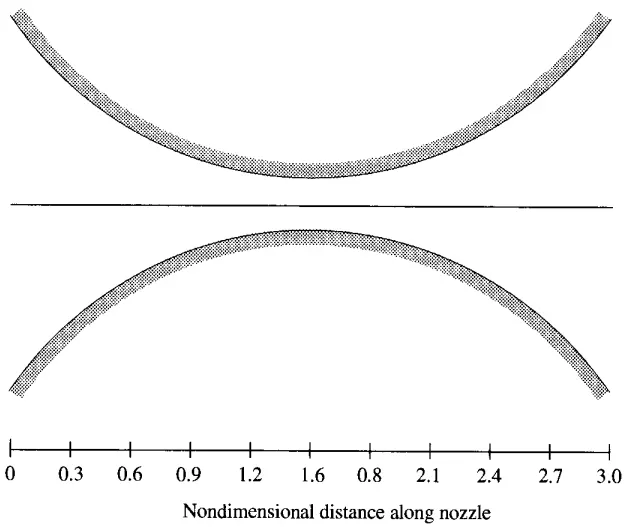
Initial Condition for Area,

`\begin{equation} A=1+2.2(x-1.5)^{2} \quad 0 \leq x \leq 3 \end{equation}`

Initial Conditions for density, velocity, temperature are given as follows:

`\begin{equation} \begin{aligned} &\rho=1-0.3146 x \\ &T=1-0.2314 x \\ &V=(0.1+1.09 x) T^{1 / 2} \end{aligned} \end{equation}`

This concludes the NON-CONSERVATION FORM OF THE DERIVATION.

==============================================================================

CONSERVATION FORM:

Continuity:

`\begin{equation} \frac{\partial(\rho A)}{\partial t}+\frac{\partial(\rho A V)}{\partial x}=0 \end{equation}`

In Non-Dimentional form,

`\begin{equation} \frac{\partial\left(\rho^{\prime} A^{\prime}\right)}{\partial t^{\prime}}+\frac{\partial\left(\rho^{\prime} A^{\prime} V^{\prime}\right)}{\partial x^{\prime}} \end{equation}`

Momentum:

`\begin{equation} \frac{\partial(\rho A V)}{\partial t}+\frac{\partial\left(\rho A V^{2}\right)}{\partial x}=-A \frac{\partial p}{\partial x} \end{equation}`

In Non-Dimentional form,

`\begin{equation} \frac{\partial\left(\rho^{\prime} A^{\prime} V^{\prime}\right)}{\partial t^{\prime}}+\frac{\partial\left[\rho^{\prime} A^{\prime} V^{\prime 2}+(1 / \gamma) p^{\prime} A^{\prime}\right]}{\partial x^{\prime}}=\frac{1}{\gamma} p^{\prime} \frac{\partial A^{\prime}}{\partial x^{\prime}} \end{equation}`

Energy:

`\begin{equation} \frac{\partial\left[\rho\left(e+V^{2} / 2\right) A\right]}{\partial t}+\frac{\partial\left[\rho\left(e+V^{2} / 2\right) A V\right]}{\partial x}=-\frac{\partial(p A V)}{\partial x} \end{equation}`

In Non-Dimentional form,

`\begin{equation} \frac{\partial\left[\rho^{\prime}\left(\frac{e^{\prime}}{\gamma-1}+\frac{\gamma}{2} V^{\prime 2}\right) A^{\prime}\right]}{\partial t^{\prime}}+\frac{\partial\left[\rho^{\prime}\left(\frac{e^{\prime}}{\gamma-1}+\frac{\gamma}{2} V^{\prime 2}\right) V^{\prime} A^{\prime}+p^{\prime} A^{\prime} V^{\prime}\right]}{\partial x^{\prime}}=0 \end{equation}`

In the conservation form the governing equations are expressed in terms of solution vector, flux vector and source terms if any. They are given as follows:

`\begin{equation} \begin{aligned} &U_{1}=\rho^{\prime} A^{\prime} \\ &U_{2}=\rho^{\prime} A^{\prime} V^{\prime} \\ &U_{3}=\rho^{\prime}\left(\frac{e^{\prime}}{\gamma-1}+\frac{\gamma}{2} V^{\prime 2}\right) A^{\prime} \\ &F_{1}=\rho^{\prime} A^{\prime} V^{\prime} \\ &F_{2}=\rho^{\prime} A^{\prime} V^{\prime 2}+\frac{1}{\gamma} p^{\prime} A^{\prime} \\ &F_{3}=\rho^{\prime}\left(\frac{e^{\prime}}{\gamma-1}+\frac{\gamma}{2} V^{\prime 2}\right) V^{\prime} A^{\prime}+p^{\prime} A^{\prime} V^{\prime} \\ &J_{2}=\frac{1}{\gamma} p^{\prime} \frac{\partial A^{\prime}}{\partial x^{\prime}} \end{aligned} \end{equation}`

Therefore governing equation takes the form,

`\begin{equation} \begin{aligned} &\frac{\partial U_{1}}{\partial t^{\prime}}=-\frac{\partial F_{1}}{\partial x^{\prime}} \\ &\frac{\partial U_{2}}{\partial t^{\prime}}=-\frac{\partial F_{2}}{\partial x^{\prime}}+J_{2} \\ &\frac{\partial U_{3}}{\partial t^{\prime}}=-\frac{\partial F_{3}}{\partial x^{\prime}} \end{aligned} \end{equation}`

Primitive variables are expressed in terms of U1, U2, U3

`\begin{equation} \begin{aligned} \rho^{\prime} &=\frac{U_{1}}{A^{\prime}} \\ V^{\prime} &=\frac{U_{2}}{U_{1}} \\ T^{\prime} &=e^{\prime}=(\gamma-1)\left(\frac{U_{3}}{U_{1}}-\frac{\gamma}{2} V^{\prime 2}\right) \\ p^{\prime} &=\rho^{\prime} T^{\prime} \end{aligned} \end{equation}`

As seen above, F1, F2, F3 are expressed in terms of density, velocity and temperature. It was found that solving the flux vectors in terms of primitive variables, the computer code becomes unstable after some time step. So the best pratice to avoid such an instability, the flux vectores are expressed in the purest form ie. in the form of U1, U2, U3.

F1, F2, F3 are given as follows:

F1,

`\begin{equation} F_{1}=U_{2} \end{equation}`

F2,

`\begin{equation} F_{2}=\frac{U_{2}^{2}}{U_{1}}+\frac{\gamma-1}{\gamma}\left(U_{3}-\frac{\gamma}{2} \frac{U_{2}^{2}}{U_{1}}\right) \end{equation}`

F3,

`\begin{equation} F_{3}=\gamma \frac{U_{2} U_{3}}{U_{1}}-\frac{\gamma(\gamma-1)}{2} \frac{U_{2}^{3}}{U_{1}^{2}} \end{equation}`

J2,

`\begin{equation} J_{2}=\frac{\gamma-1}{\gamma}\left(U_{3}-\frac{\gamma}{2} \frac{U_{2}^{2}}{U_{1}}\right) \frac{\partial\left(\ln A^{\prime}\right)}{\partial x^{\prime}} \end{equation}`

BOUNDARY CONDITIONS:

At the subsonic inflow boundary condition two properties are held fixed and one is allowed to float (allowed to vary with time).

At the supersonic outflow boundary condition all the properties are allowed to float.

At inflow,

`\begin{equation} U_{1(i=1)}=\left(\rho^{\prime} A^{\prime}\right)_{i=1}=A_{i=1}^{\prime}=\text { fixed value } \end{equation}`

`\begin{equation} U_{2(i=1)}=2 U_{2(i=2)}-U_{2(i=3)} \end{equation}`

`\begin{equation} U_{3}=U_{1}\left(\frac{T^{\prime}}{\gamma-1}+\frac{\gamma}{2} V^{\prime 2}\right) \end{equation}`

At outflow,

`\begin{equation} \begin{aligned} &\left(U_{1}\right)_{N}=2\left(U_{1}\right)_{N-1}-\left(U_{1}\right)_{N-2} \\ &\left(U_{2}\right)_{N}=2\left(U_{2}\right)_{N-1}-\left(U_{2}\right)_{N-2} \\ &\left(U_{3}\right)_{N}=2\left(U_{3}\right)_{N-1}-\left(U_{3}\right)_{N-2} \end{aligned} \end{equation}`

INITIAL CONDITIONS:

`\begin{equation} \begin{aligned} &\left.\begin{array}{l} \rho^{\prime}=1.0 \\ T^{\prime}=1.0 \end{array}\right\} \text { for } 0 \leq x^{\prime} \leq 0.5\\ &\left.\begin{array}{l} \rho^{\prime}=1.0-0.366\left(x^{\prime}-0.5\right) \\ T^{\prime}=1.0-0.167\left(x^{\prime}-0.5\right) \end{array}\right\} \text { for } 0.5 \leq x^{\prime} \leq 1.5\\ &\left.\begin{array}{l} \rho^{\prime}=0.634-0.3879\left(x^{\prime}-1.5\right) \\ T^{\prime}=0.833-0.3507\left(x^{\prime}-1.5\right) \end{array}\right\} \text { for } 1.5 \leq x^{\prime} \leq 3.5 \end{aligned} \end{equation}`

`\begin{equation} V^{\prime}=\frac{U_{2}}{\rho^{\prime} A^{\prime}}=\frac{0.59}{\rho^{\prime} A^{\prime}} \end{equation}`

Time step calculation is similar to that of non-conservation form.

Predictor Step and Corrector Step Explanation:

• To start the calculation, we use the values of U1, U2, U3 to calculate the initial values of F1, F2, F3.
• In the predictor step the flux vectors are discritized with forward differencing.
• Once the flux vectors are calculated, using this information we can calculate the values of U1, U2, U3. Once we know U1, U2, U3 we update the values of the primitive variables.
• Once we have updated the values of primitive variables , we again calculate the values of F1, F2, F3 or in other words we update the values of F1, F2, F3.
• These values of F1, F2, F3 will help us to calculate the corrector step. In corrector step the flux vectors are discritized with rearward differencing.
• Now we calculate the average time derivative followed by updating the values of U1, U2, U3 and obtaining the final values of the primitive variables.

This concludes the CONSERVATION FORM derivation.

==============================================================================

CODE FOR CONSERVATION AND NON-CONSERVATION FORM:

%% ========== NON-CONSERVATION FORM ========== %%

% This is the NON CONSERVATION FORM OF GOVERNING EQUATION FOR QUASI 1D
% SUBSONIC SUPERSONIC ISENTROPIC NOZZLE FLOW

function [rho ,v ,t, m_dot_th] = one_D_non_conservation(n,nt)
% Inputs
x = linspace(0,3,n);
dx = x(2)- x(1);
gamma = 1.4;

% Calcuate Initial Profiles
rho = 1-0.3146*x;
t = 1-0.2314*x; % t = Temperature
v = (0.1+1.09*x).*t.^0.5;

% Area
a = 1+2.2*(x-1.5).^2;   

% Time step
% dt = 0.0201;
 courant_number = 0.5;
 for d = 1:n
    d_t(d) = courant_number*(dx/((sqrt(t(d))) + v(d))); 
    
 end
dt = min(min(d_t));

% Outer time loop
for k = 1:nt
    
      rho_old = rho;
      v_old = v;
      t_old = t;
      
   % Predictor Method
   
    for j = 2:n-1
       dvdx = (v(j+1) - v(j))/dx;
       drhodx = (rho(j+1) - rho(j))/dx;
       dtdx = (t(j+1) - t(j))/dx;
       dlogadx = (log(a(j+1)) - log(a(j)))/dx;  
       
       % Continuity Equation
       drhodt_p(j) = -rho(j)*dvdx - rho(j)*v(j)*dlogadx - v(j)*drhodx;
       
       % Momentum Equation 
       dvdt_p(j) = -v(j)*dvdx - (1/gamma)*(dtdx + (t(j)/rho(j))*drhodx);
       
       % Energy Equation
       dtdt_p(j) = -v(j)*dtdx - (gamma-1)*t(j)*(dvdx + v(j)*dlogadx);
       
       
       % Solution Update 
       rho(j) = rho(j) + drhodt_p(j)*dt;
       v(j) = v(j) + dvdt_p(j)*dt;
       t(j) = t(j) + dtdt_p(j)*dt;
        
    end
    
    
    % Corrector Method
    
    for j = 2:n-1
       dvdx = (v(j) - v(j-1))/dx;
       drhodx = (rho(j) - rho(j-1))/dx;
       dtdx = (t(j) - t(j-1))/dx;
       dlogadx = (log(a(j)) - log(a(j-1)))/dx;
       
       % Continuity Equation
       drhodt_c(j) = -rho(j)*dvdx - rho(j)*v(j)*dlogadx - v(j)*drhodx;
       
       % Momentum Equation 
       dvdt_c(j) = -v(j)*dvdx - (1/gamma)*(dtdx + (t(j)/rho(j))*drhodx);
       
       % Energy Equation
       dtdt_c(j) = -v(j)*dtdx - (gamma-1)*t(j)*(dvdx + v(j)*dlogadx);
             
    end
    
       % Compute the average time derivative
       drhodt = 0.5*(drhodt_p + drhodt_c);
       dvdt = 0.5*(dvdt_p + dvdt_c);
       dtdt = 0.5*(dtdt_p + dtdt_c);
       
       % Final Solution Update 
       for i = 2:n-1
           rho(i) = rho_old(i) + drhodt(i)*dt;
           v(i) = v_old(i) + dvdt(i)*dt;
           t(i) = t_old(i) + dtdt(i)*dt;
       end
       
       % Apply the Boundary Conditions 
       % Inlet
       v(1) = 2*v(2) - v(3);
       
       % Outlet
       v(n) = 2*v(n-1) - v(n-2);
       rho(n) = 2*rho(n-1) - rho(n-2);
       t(n) = 2*t(n-1) - t(n-2);
       
       % Mass Flow Rate
       l= find(a==min(a));
       m_dot(k,:) = rho.*v.*a;
       m_dot_th(k) = m_dot(l);
       
       % Plotting primitive variables at throat section  
         
         rho_th(k) = rho(l);
         figure(1)
         plot(rho_th)
         title(sprintf('Time Step = %d',k))
         xlabel('Time Step')
         ylabel('Density at Throat')
         pause(0.03)
         
         v_th(k) = v(l);
         figure(2)
         plot(v_th)
         title(sprintf('Time Step = %d',k))
         xlabel('Time Step')
         ylabel('Velocity at Throat')
         pause(0.03)
         
         t_th(k) = t(l);
         figure(3)
         plot(t_th)
         title(sprintf('Time Step = %d',k))
         xlabel('Time Step')
         ylabel('Temperature at Throat')
         pause(0.03)
       
       
        
end
        % Plotting
        figure(4)
        plot(x,rho)
        title(sprintf('Time Step = %d',k))
        xlabel('X-axis')
        ylabel('Non-Dimentional Density')
       
        figure(5)
        plot(x,v)
        title(sprintf('Time Step = %d',k))
        xlabel('X-axis')
        ylabel('Non-Dimentional Velocity')
       
        figure(6)
        plot(x,t)
        title(sprintf('Time Step = %d',k))
        xlabel('X-axis')
        ylabel('Non-Dimentional Temperature')
        
        % Plotting of variation of Mass Flow Rate at different time step
        figure(7)
        plot(x,m_dot(700,:),'r')
        hold on
        plot(x,m_dot(200,:),'b')
        hold on
        plot(x,m_dot(100,:),'g')
        xlabel('X-Axis')
        ylabel('Non-Dimentional Mass Flow Rate')
        legend('700dt','200dt','100dt')

end

%% ========== CONSERVATION FORM ========== %%

% This is the CONSERVATION FORM OF GOVERNING EQUATION FOR QUASI 1D
% SUBSONIC SUPERSONIC ISENTROPIC NOZZLE FLOW

function [rho ,v ,t, m_dot_th] = one_D_conservation(n,nt)
% Inputs
x = linspace(0,3,n);
dx = x(2)- x(1);
gamma = 1.4;


% INITIAL CONDITIONS FOR
% Area
a = 1+2.2*(x-1.5).^2;
% Density (rho)
rho = ones(1,n);
t = ones(1,n); % t = TEMPERATURE
for i = 1:length(x)
    if x(i)>= 0 && x(i)<= 0.5
        rho(i) = 1;
        t(i) = 1;
    end
end
for i = 1:length(x)
    if x(i)>= 0.5 && x(i)<=1.5
        rho(i) = 1-0.366*(x(i)-0.5);
        t(i) = 1-0.167*(x(i)-0.5);
    end
end
for i = 1:length(x)
    if x(i)>= 1.5 && x(i)<=3
        rho(i) = 0.634-0.3879*(x(i)-1.5);
        t(i) = 0.833-0.3507*(x(i)-1.5);
    end
end

% Velocity
v = 0.59./(rho.*a);


% copy of rho v and t
rho_old = rho;
t_old = t;
v_old = v;


% Calculating SOLUTION VECTOR U1 ,U2, U3.
u1 = rho.*a;
u2 = rho.*a.*v;
u3 = u1.*((t./(gamma-1))+((gamma/2).*(v.^2)));



% dt = 0.0267;
courant_number = 0.5;
for d = 1:n
   d_t(d) = courant_number*(dx/((sqrt(t(d))) + v(d)));    
end
dt = min(d_t);

for k = 1:nt
    u1_old = u1;
    u2_old = u2;
    u3_old = u3;
    
    % Calculating f1,  f2, f3
    for b = 1:n
        % for f1 calculation 
        f1(b) = u2(b);
    
        % for f2 calculation
        f2(b) = ((u2(b).^2)./u1(b)) + (((gamma-1)/gamma)*(u3(b) - ((gamma/2)*((u2(b).^2)./u1(b)))));
    
        % for f3 calculation
        f3(b) = ((gamma)*((u2(b).*u3(b))./u1(b))) - (((gamma*(gamma-1))/2)*((u2(b).^3)./(u1(b).^2)));
       
    end


    % Predictor Step
    for c = 2:n-1
        du1dt_p(c) = - ((f1(c+1)-f1(c))/dx); 
        du2dt_p(c) = - ((f2(c+1)-f2(c))/dx) +  (1/gamma)*(rho(c).*t(c).*((a(c+1)-a(c))/dx));
        du3dt_p(c) = - ((f3(c+1)-f3(c))/dx);
    
        % Update values of u1, u2, u3
        u1(c) = u1(c) + du1dt_p(c)*dt;
        u2(c) = u2(c) + du2dt_p(c)*dt;
        u3(c) = u3(c) + du3dt_p(c)*dt;
        
        % Update value of primitive variables
        rho(c) = u1(c)./a(c);
        v(c) = u2(c)/u1(c);
        t(c) = (gamma-1)*((u3(c)./u1(c))-((gamma/2)*((v(c).^2))));
    end
    
    % Calculating f1,  f2, f3
    for b = 1:n
        % for f1 calculation 
        f1c(b) = u2(b);
    
        % for f2 calculation
        f2c(b) = ((u2(b).^2)./u1(b)) + (((gamma-1)/gamma)*(u3(b) - ((gamma/2)*((u2(b).^2)./u1(b)))));
    
        % for f3 calculation
        f3c(b) = ((gamma)*((u2(b).*u3(b))./u1(b))) - (((gamma*(gamma-1))/2)*((u2(b).^3)./(u1(b).^2)));
       
    end
    
    % Corrector Method
    for c = 2:n-1
        du1dt_c(c) = - ((f1c(c)-f1c(c-1))/dx); 
        du2dt_c(c) = - ((f2c(c)-f2c(c-1))/dx) +  (1/gamma)*(rho(c).*t(c).*((a(c)-a(c-1))/dx));
        du3dt_c(c) = - ((f3c(c)-f3c(c-1))/dx);
           
    end
    
    % Compute the average time derivative
      du1dt = 0.5.*(du1dt_p + du1dt_c);
      du2dt = 0.5.*(du2dt_p + du2dt_c);
      du3dt = 0.5.*(du3dt_p + du3dt_c);
      
     for c = 2:n-1
         % Update values of u1, u2, u3
        u1(c) = u1_old(c) + du1dt(c)*dt;
        u2(c) = u2_old(c) + du2dt(c)*dt;
        u3(c) = u3_old(c) + du3dt(c)*dt; 
     end
      
      % Boundary Conditions
      % Inlet
      u1(1) =  rho(1)*a(1);
      u2(1) =  2*u2(2)-u2(3);
%     v(1) =   u2(1)/u1(1);
      u3(1) =  u1(1).*((t(1)./(gamma-1))+((gamma/2).*(v(1).^2)));
      
      % outlet
      u1(n) = 2*u1(n-1) - u1(n-2);
      u2(n) = 2*u2(n-1) - u2(n-2);
      u3(n) = 2*u3(n-1) - u3(n-2);
      
      rho = u1./a;
      v = u2./u1;
      t = (gamma-1)*((u3./u1)-((gamma/2)*((v.^2))));
      
      % Mass Flow Rate
      l= find(a==min(a));
      m_dot(k,:) = rho.*v.*a;
      m_dot_th(k) = m_dot(l);
      
       
         % Plotting primitive variables at throat section  
         
         rho_th(k) = rho(l);
         figure(8)
         plot(rho_th)
         title(sprintf('Time Step = %d',k))
         xlabel('Time Step')
         ylabel('Density at Throat')
         pause(0.03)
         
         v_th(k) = v(l);
         figure(9)
         plot(v_th)
         title(sprintf('Time Step = %d',k))
         xlabel('Time Step')
         ylabel('Velocity at Throat')
         pause(0.03)
         
         t_th(k) = t(l);
         figure(10)
         plot(t_th)
         title(sprintf('Time Step = %d',k))
         xlabel('Time Step')
         ylabel('Temperature at Throat')
         pause(0.03)
     
end

% Plotting of variation of Mass Flow Rate at different time step
figure(11)
plot(x,m_dot(700,:),'r')
hold on
plot(x,m_dot(200,:),'b')
hold on
plot(x,m_dot(100,:),'g')
xlabel('X-Axis')
ylabel('Non-Dimentional Mass Flow Rate')
legend('700dt','200dt','100dt')

% Plotting Steady State distribution of primitive variables
figure(12)
plot(x,rho)
title(sprintf('Time Step = %d',k))
xlabel('X-axis')
ylabel('Non-Dimentional Density')
       
figure(13)
plot(x,v)
title(sprintf('Time Step = %d',k))
xlabel('X-axis')
ylabel('Non-Dimentional Velocity')
       
figure(14)
plot(x,t)
title(sprintf('Time Step = %d',k))
xlabel('X-axis')
ylabel('Non-Dimentional Temperature')

end

%% ========== MAIN CODE ========== %%

n = input('Enter Number of Grid point: ');
nt = input('Enter Number of Time steps: ');
x = linspace(0,3,n);
% Area
a = 1+2.2*(x-1.5).^2;

% Calling the function
[rho_nc ,v_nc ,t_nc, m_dot_nc_th] = one_D_non_conservation(n,nt);
[rho_c ,v_c ,t_c, m_dot_c_th] = one_D_conservation(n,nt);

figure(15)
plot(x,(rho_nc.*v_nc.*a))
hold on
plot(x,(rho_c.*v_c.*a))
xlabel('X-Axis')
ylabel('Non-dimentionalized Density')
legend('Non-Conservation','Conservation')

CODE EXPLANATION:

Non-Conservation Form:

• Length of the nozzle is 3 units and it is divided into n number of grid points. Number of grid points is specified by the user in the main code.
• We have calculated the initial profile for the primitive variables. (refer John Anderson)
• Time step is decided with the help of courant number and is chosen to be the minimum value.
• Outer loop is the time loop.
• We have creadted a copy of primitive variables to make out the difference between the updated and the initial values.
• Starting with the predictor method, the code is divided into simple steps for ease of coding and fast error checking. All the terms with spatial derivative are discritized with forward differencing.
• Later, the soulution is updated, meaning, we update the primitive variables of the governing equation.
• After updating the primitive variables, these are used in calculating the corrector step. In corrector step, all the terms with spatial derivative are dicritized with rearward differencing.
• Average time derivative is calculated once we have evaluated the predicted values and corrected values.
• Finally, we updated the primitive variables.
• It is always necessary to provide boundary condition in order to procede with the solution and arrive at correct values of the flow field.
• Last, the plotting is done for intuitive information extraction.

==============================================================================

Conservation Form:

• Length of the nozzle is same 3 units and is divided into N number of grid points.
• The initial profile is different from what we saw in non-conservation form. This is to make the profile more closer to the expeted result so as to reduce error and converge at a faster rate. Note, we can give arbitary guess value, which will take or might take lot of time to converge.
• Time step calculation is similar to that of non-conservation form.
• Outer loop is the time loop.
• In conservation form the governing equations are expressed in terms of solution vector, flux vector and source term if any.
• The governing equation are entirely in terms of U1, U2, U3 and in non-dimentional form. This is to make sure that the solution is in its pure form and keeps the code stable.
• First we calculate the values of F1, F2, F3 which are interms of U1, U2, U3.
• Entering into the predictor step, the spatial derivatives are discritized with forward differencing.
• We update the values of U1, U2, U3 and following to it we update the value of primitive variables.
• Since we have updated the values of primitive variables, we now must updated the values of F1, F2, F3.
• These updated values are now used in the corrector step, where, the terms with spatial derivative are discritized with rearward differencing.
• Average time derivative is calculated followed by updating the values of U1, U2, U3 and then finally updating the values of the primitive variables.
• Last, the plotting is done for intuitive information extraction.
  

GRID INDEPENDENCE STUDY:

• When there is no change in the values of the flow field after reducing the grid spacing between the node or increasing the number of nodes for given size of domain, we can say that we have arrived at grid independence and on furthur increasing of number of nodes will not change the result.
• What we observed is, grid independence is achieved at the number of nodes = 31, for conservation form. It really does not have any effect on results after increasing the grid points.

COMPARISON OF NON-CONSERVATION FORM AND CONSERVATION FORM:

• Conservation form yields better mass flow distribution.
• Non- conservation form gives smaller residual values.
• Non- conservation form produces better results for primitive variables and conservation form produces better results for flux vector variables.

Reference: CFD book by John Anderson.