Week 4.1: Project - Steady state simulation of flow over a throttle body

Aim: To simulate flow insidde a throttle body.

Take away:

By the end of this article, one will be able to,

• Import CAD file of .STL format into Converge Studio.
• Assign boundary flagging.
• Set up the case.
• Export the necessary output files.
• Run the simulation using Cygwin.
• Post process the results using Paraview.

==============================================================================

Theory:

• In fuel injected engines, the throttle body is the part of the air intake system that controls the amount of air flowing into the engine, in response to driver accelerator pedal input in the main.
• The throttle body is usually located between the air filter box and the intake manifold, and it is usually attached to, or near, the mass airflow sensor.
• Often, an engine coolant line also runs through it in order for the engine to draw intake air at a certain temperature (the engine's current coolant temperature, which the ECU senses through the relevant sensor) and therefore with a known density.
• The largest piece inside the throttle body is the throttle plate, which is a butterfly valve that regulates the airflow.
• On many cars, the accelerator pedal motion is communicated via the throttle cable, which is mechanically connected to the throttle linkages, which, in turn, rotate the throttle plate.

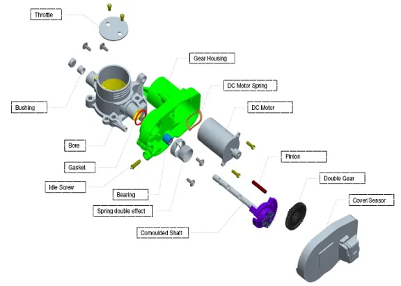
• In cars with electronic throttle control (also known as "drive-by-wire"), an electric actuator controls the throttle linkages and the accelerator pedal connects not to the throttle body, but to a sensor, which outputs a signal proportional to the current pedal position and sends it to the ECU.
• When the driver presses on the accelerator pedal, the throttle plate rotates within the throttle body, opening the throttle passage to allow more air into the intake manifold, immediately drawn inside by its vacuum.
• Usually a mass airflow sensor measures this change and communicates it to the ECU.
• The ECU then increases the amount of fuel injected by the injectors in order to obtain the required air-fuel ratio.
• Often a throttle position sensor (TPS) is connected to the shaft of the throttle plate to provide the ECU with information on whether the throttle is in the idle position, wide-open throttle (WOT) position, or somewhere in between these extremes.
• The ECU then determines the throttle opening based on the accelerator pedal's position and inputs from other engine sensors such as the engine coolant temperature sensor.

Reference: Link

==============================================================================

Import Geometry:

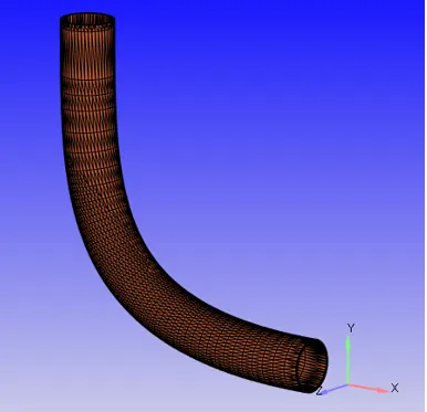
• Navigate to the "Files", then select "Import" and then select "Import STL".
• An easy was is to just drag and drop the STL file into the graphics area.

Geometry Cleanup:

• In this simulation we are not trying to simulate conjugate heat transfer, so, we can remove the thickness of the pipe.
• Make sure in the "By Angle" selection mode.

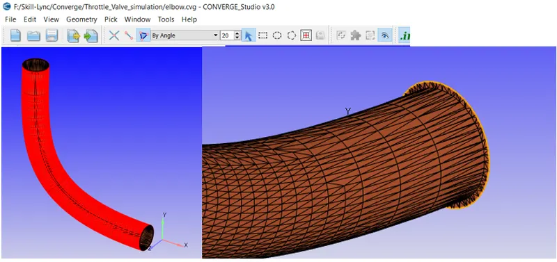
• The above image shows that the outer surface of the pipe is deleted and is no more required for simulation.
• Similarly remove the remaining two surface which are perpendicular to the inner pipe surface.
• After which you will end up with the geometry as shown below:

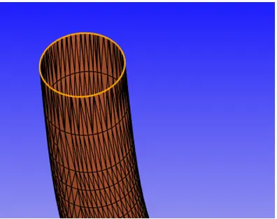
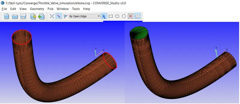
• Next step would be to patch the open ends of the geometry.
• Navigate to "Repair", then select "Patch", then pick "Free open edges".
• Make sure you have selected the right selection filter. "By open edge".
• After executing this command, now the geometry is closed and ready for setup.

Diagnostics:

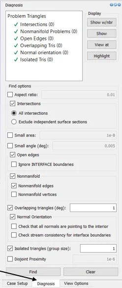
• Find this tab at the right bottom corner of the view port.
• Make sure there are no errors present in the geometry.

Boundary Flagging:

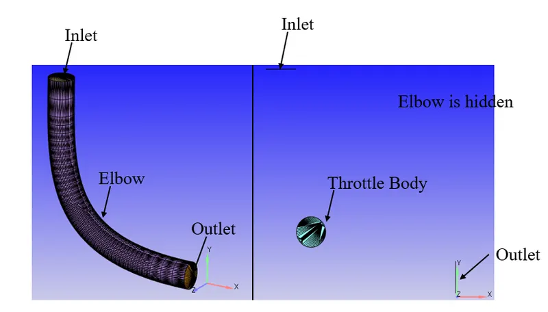
• Navigate to "Boundary". Present in "Geometry Dock".
• Click on "+" icon to add boundaries to be flagged.
• Refer to the below figure to flag the boundary.

Case setup:

• Click on "Begin case setup".
• By clicking, one needs to set the appropriate boundary conditions and all the other parameters for replicating the physics.

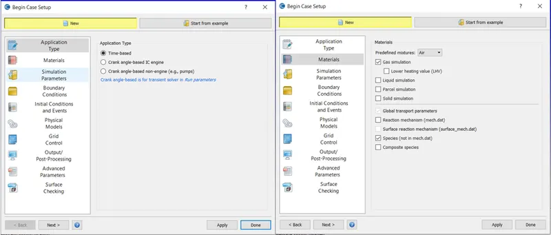
• Select "Time-based" in "Application Type".
• Select Materials, "Predefined mixture: Air". Check "Gas simulation","Species" and uncheck "Species".
• Hit "Apply" and then "Done".

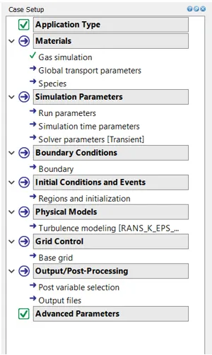
• Once the above step is done, you will be greeted with the following options as shown in the figure below.
• Complete all the steps to setup the simulation.

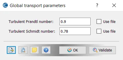
• Select "Global Transport properties".
• Keep the values as default.

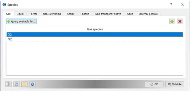
• Select "Species".
• Add O2 and N2 to the list by clicking on "+" icon.

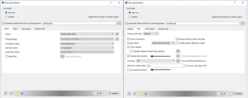
• Select "Run Parameters".
• Temporal type: Steady-State solver
• Check "Steady state monitor". Uncheck "Use shared memory".

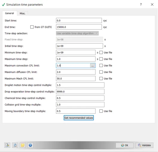
• Select "Simulation time parameters".
• End time: 15,000 cyc.
• Initial time-step: 1e-09
• Minimum time-step: 1e-09
• Maximum convection CFL limit: 1
• Rest as default.

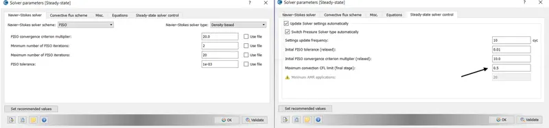
• Select "Solver-parameters".
• Make sure "Maximum convection CFL limit" is 0.5

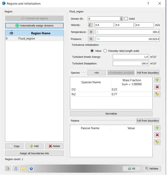
• Select "Region and initialization".
• Create a region by clicking on "+" icon.
• Refer the figure below.

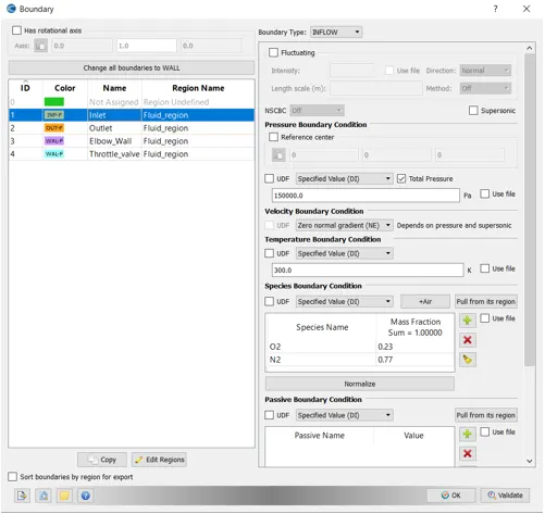
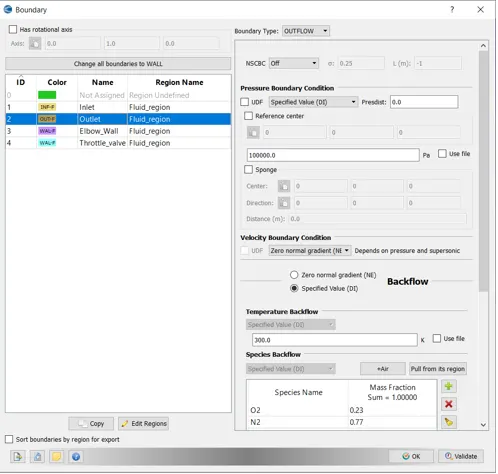
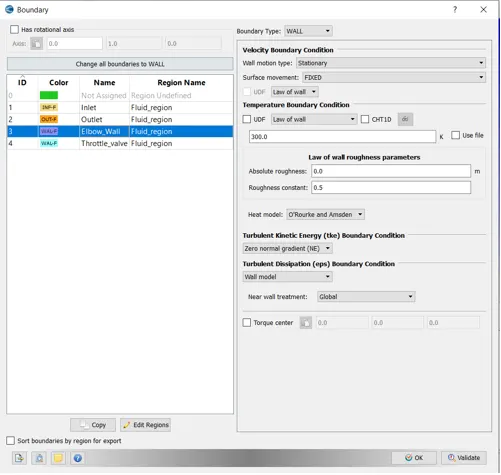
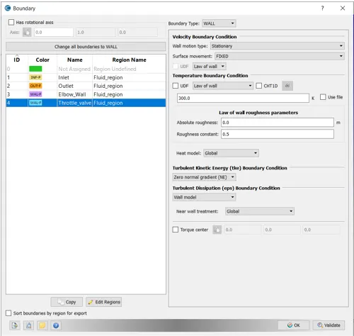
• Select "Boundary".

1) Inlet:

2) Outlet:

3) Elbow_Wall:

4) Throttle_valve:

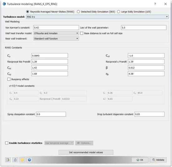
• Select "Turbulence Modelling".
• Set all the values as default.

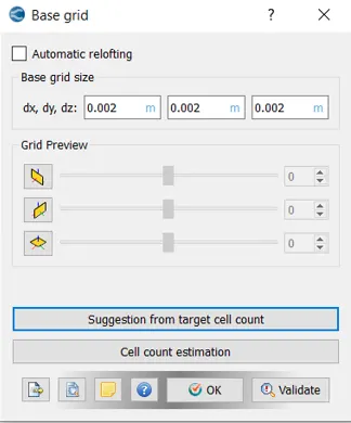
• Select "Base Grid".
• Mesh size: 0.002,0.002,0.002 m in x,y,z directions respectively.

• Select "Grid Control".

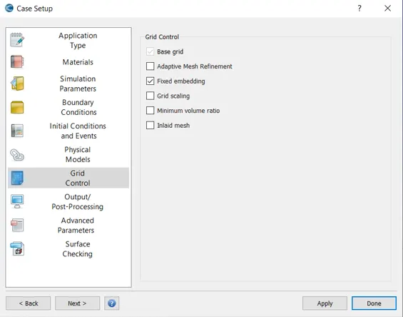
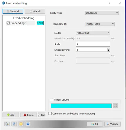
• Enable "Fixed Embedding".
• Make sure "Entity type" is set "BOUNDARY".
• "Boundary ID" is set to "Throttle_valve". Since we need a finer mesh near the throttle valve.
• "Scale" is 3 and "Embed Layers" is 2. One can play around and fine tune the mesh to observe changes in results.

==============================================================================

How to run simulation:

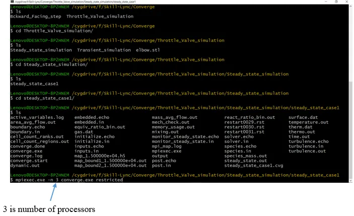
• Export the input files. Navigate to "Files > Export > Export input files".
• Export the files to a folder.
• Run "Cygwin" as administrator.
• Navigate to the folder where the input files are dumped.
• Run the simulation by typing the command, mpiexec.exe -n converge.exe restricted.
• Make sure you have two files in the same folder as the input files "mpiexec.exe" and "converge.exe"

==============================================================================

Results:

Results from CONVERGE:

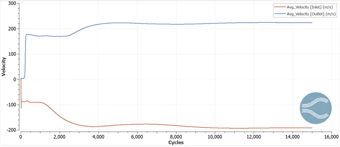
• Velocity Plot:

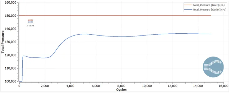
• Total Pressure Plot:

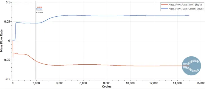
• Mass Flow Rate Plot:

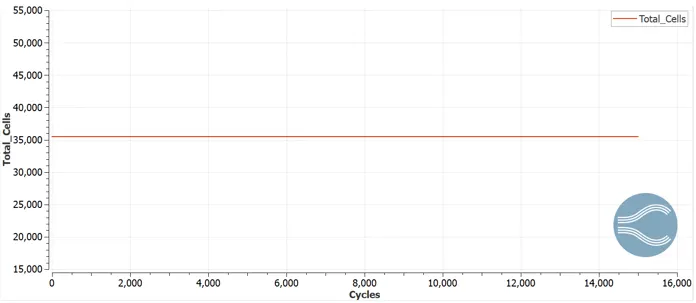
• Total Mesh Count:

Results from Paraview:

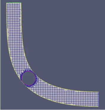
• Mesh:

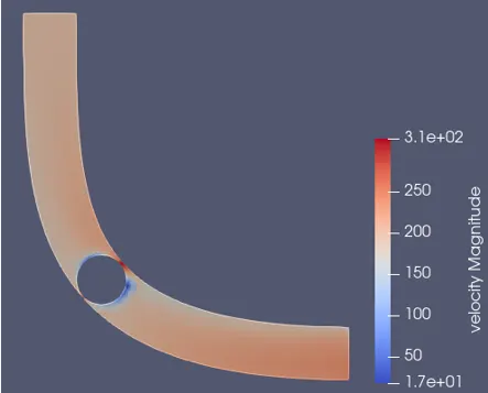
• Velocity Contour:

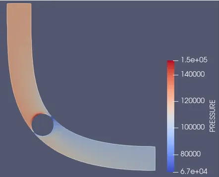
• Pressure Contour:

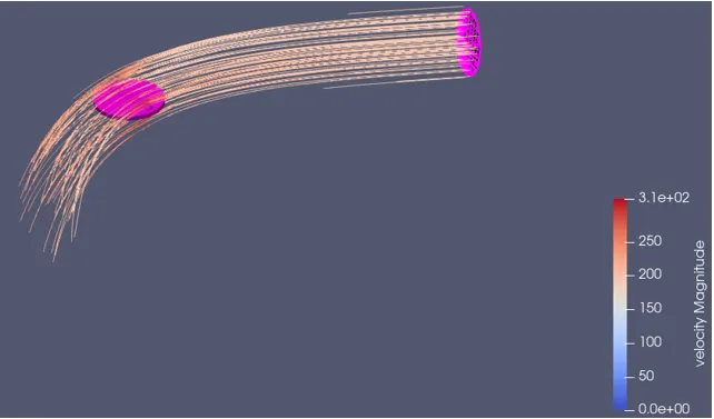
• Streamlines:

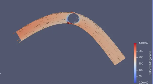
• Vectors:

==============================================================================

Conclusion:

• Velocity at the edges of the throttle valve is high.
• Pressure at the face of the throttle valve is high and forms stagnation point.
• Velocity at this location is zero or close to zero as the flow faces an obsturction which casues rise in stagnation pressure.