Week 4 - CHT Analysis on Exhaust port

Aim: To understand the concept of Conjugate Heat Transfer and its applictions in the industry.

===============================================================================

Q1. Give a brief description of why and where a CHT analysis is used.

• Conjugate heat transfer (CHT) analysis can accurately predict heat transfer by simultaneous solving all the relevant solid and flow field heat transfer processes.
• This model, based on a strictly mathematically stated problem, describes the heat transfer between a body and a fluid flowing over or inside it as a result of the interaction of two objects.
• The physical processes and solutions of the governing equations are considered separately for each object in two subdomains.
• Matching conditions for these solutions at the interface provide the distributions of temperature and heat flux along the body–flow interface, eliminating the need for a heat transfer coefficient. Moreover, it may be calculated using these data.
• Applications: Gas turbine, Internal Combustion engine, aerospace industry, automobile industry, electronics cooling etc.
• In incompressible flows the energy equation is decoupled from the momentum equations and can be solved a posteriori with the velocity field frozen.
• Additional modeling is involved for the solution of thermal equation in the RANS context (therefore additional approximations and errors).
• Wall quantities (temperature and heat flux) are very sensitive to the modeling of near-wall turbulence.
• Conjugate heat transfer (coupled fluid/solid) are often necessary to describe accurately a physical device.
• Natural convection introduces a coupling between velocity and temperature field.

Reference: Wikipedia

Q2. Effect of `y^+` value on turbulence model.

• The Navier-Stokes equations are decomposed or in simple terms they are averaged and are know as Reynolds Average Navier Stokes equation.
• While averging, they produce an extra term, the 'Reynolds stress tensor'. We must evaluate the the reynolds stress term to close the equation.
• How is it done? This the time where turbulence model comes into picture.
• These reynolds stress tensor are related to the mean velocity gradient and the eddy viscosity (it is a fictitious term). The Reynolds stress term is calculated using Boussinesq Approximation.

Mixing Length Model and its transformation to k-epsilon model:

• We consider some distance away from the wall to incorporate the eddies under the position we considered.
• Now, if we are closer to the wall, the size of the eddies will be very small and if we are far away from wall, we might as well have large size eddies.
• `mu_(t)` was calculated as:

`mu_(t) = rho*k^(1/2)*l_(m)`

where k is constant and `l_(m)`is mixing length.

• Formula for mixing length was estimated using Prandtl Mixing length hypothesis. Given by:

`l_(m)= k*y` k=0.41

• In order to account the effect of viscosity in the viscous sub layer, the van Driest models accounts for that and is given by:

`l_(m)= k*y*[1-exp(-y^+/A^+)]` ; `A^+` = 26.0

• Since the mixing length distance is constant, the turbulence charateristics is also constant in an indirect manner. And since the turbuence is convective and diffusive in nature and not constant, this theory does not capture actual physics accurately.
• So, we solve the transport equation for turbulent kinetic energy and turbulent kinetic dissipation (k and epsilon respt.) and compute the eddey viscosity and try to close the RANS equation.
• k-epsilon model uses damping functions to take into account the viscous effect in the viscous sublayer.
• It uses `f_(1)`, `f_(2)`, and `f_(mu)` to dampen the coefficients used in the equations `C_(1)`,`C_(2)` and `C_(mu)`.
• Considering `f_(mu)`, if it is 1 then turbulent flow is dominant and if it is less than 1, then the viscous flow is dominant. Physically this lets us know how far or close are we to the wall.
• Other value, `f_(1)` and `f_(2)` dampens the coefficients `C_(1)` and `C_(2)` which are basically the production and dissipation factors of the equation.
• So in conclusion if we are using k-epsilon model for near wall analysis, it uses damping function to account viscous effects and can be used for values less than `y^+` less than 5.
• But with experiment and validation, they say that k-epsilon model is best suited for the values of `y^+` greater than or equal to 30. Which is also know as High-Reynolds Number formulation.
• Therefore, for Low-Reynolds Number formuation, k-Omega model is used. It does not use damping function to account viscous effet into the picture.

Limitations of k-epsilon model:

• It is not accurate at predicting boundary layers with advers pressure gradients. They are even worse when shocks are present.

(Link to k-omega model is referenced below for furthur understanding).

Reference 1: Fluid Mechanics 101 k-epsilon

Reference 2: Flud Mechanics 101 k-omega

==============================================================================

Simulation Procedure:

Creating Geometry:

• Geometry without fluid volume.

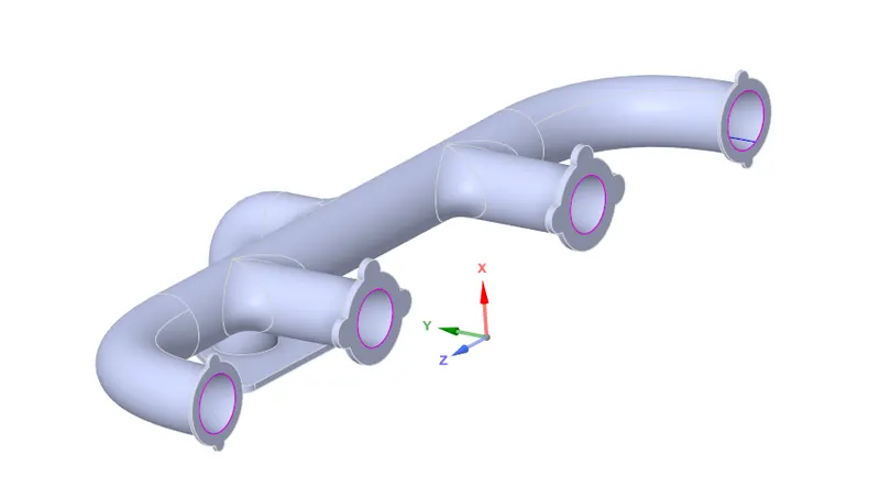
• Since we are interested in flow taking place inside the exhaust pipe, we need to create the fluid volume inside the exhaust port.
• In order to do that, navigate to prepare tab, then select 'Volume extract' option. Select edge selection and select the inner diameter of the pipe and then hit the green tick mark to create the fluid domain.
• After creating the domain, it is very much necessary to select share topology option. First select the solid body and volume extract and add them to new component and give the name as 'Final Geometry' (give any name doesn't really matter). At the end do not forget to delete empty components.
• Then select the final geometry in the tree and you must be able to see 'Share Topology' option. Change that from none to share.

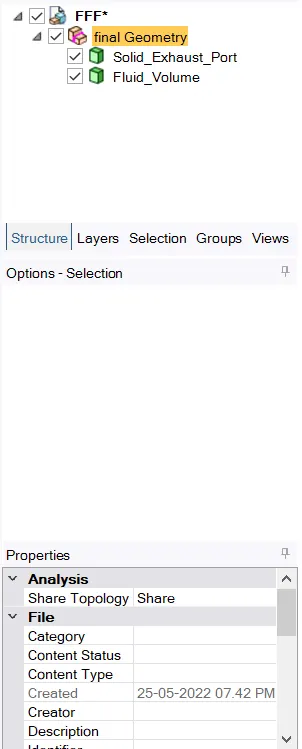
• This is the most important step; Go to Workbench tab in Spaceclaim and select 'share' option. If not done one might end up with a non conformal mesh.

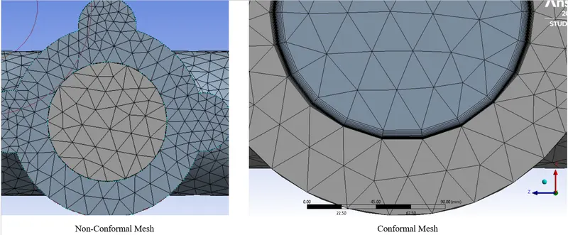
• Information does not pass properly in non-conformal mesh as compared to conformal mesh.

Creating Meshing:

• Keep the general mesh element size as 50 mm and max size as 60 mm. (find it under sizing tab).
• Select sizing (right click mesh) and select the exhaust body and assign element size of 30 mm.
• Scroll down until you find inflation option. Select the fluid surface and give name as 'inflation'. Istead of automatic selection, change it to name selection and then select 'inflation' that was created earlier.
• Select 'Total Thickness' option against Inflation option assign the values accordingly.
• Before meshing do not forget to assign named selection.

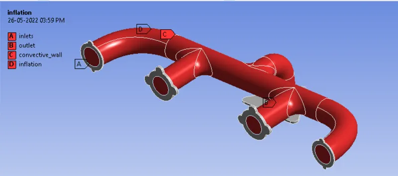
Setting up the Physics:

• Go to physics tab, select 'Energy'. For viscous, select k-epsilon model.
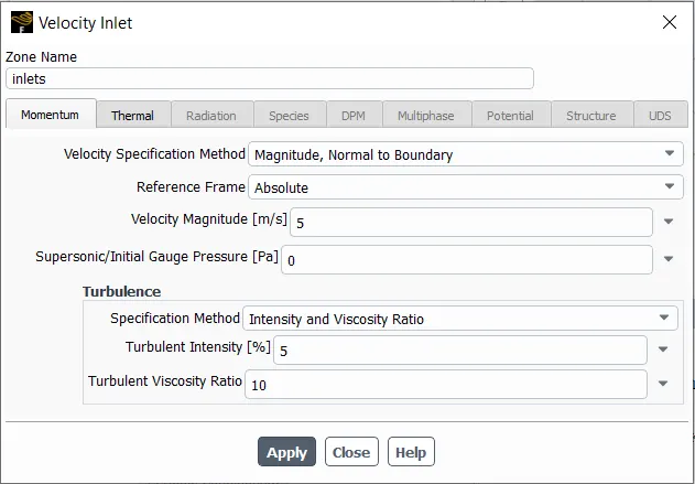
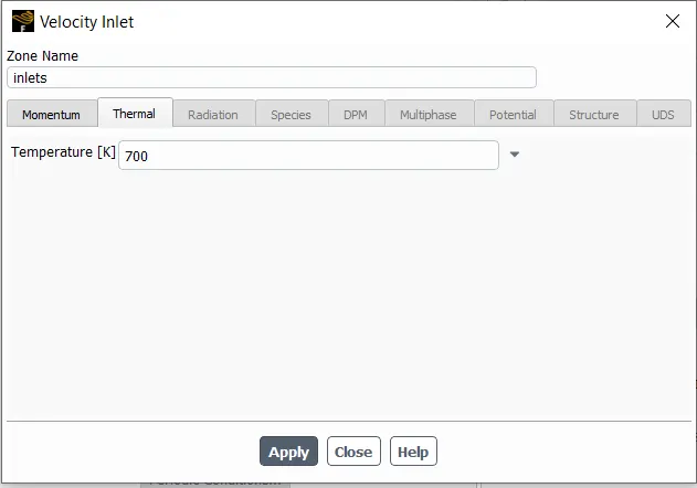
• Assign 5 m/s to inlet velocity Boundry Condition and for temperature assign 700 k.

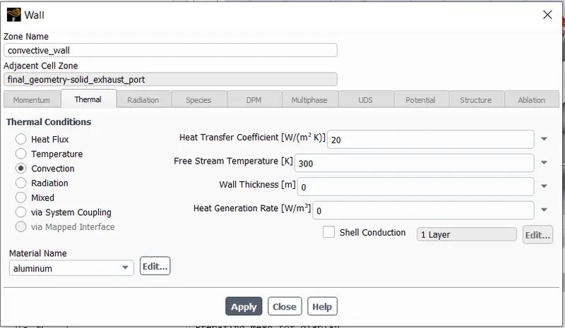
• Select convetive wall, and then select convection option and assign a value of 20 `W/(m^2*k)`

• Hybrid Initialize.
• Run calculation.

==============================================================================

Results:

Comparing the results between k-epsilon and k-omega model:

• k-epsilon:

Temperature at cut-plane:

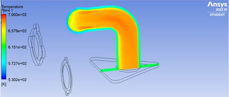
Max = 700.038 K

Min = 530.194 K

Velocity at cut plane:

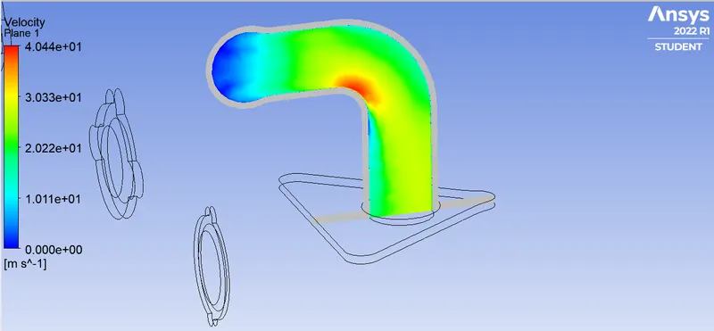
Max = 40.4369 m/s

Min = 0 m/s

Surface Heat Transfer coefficient:

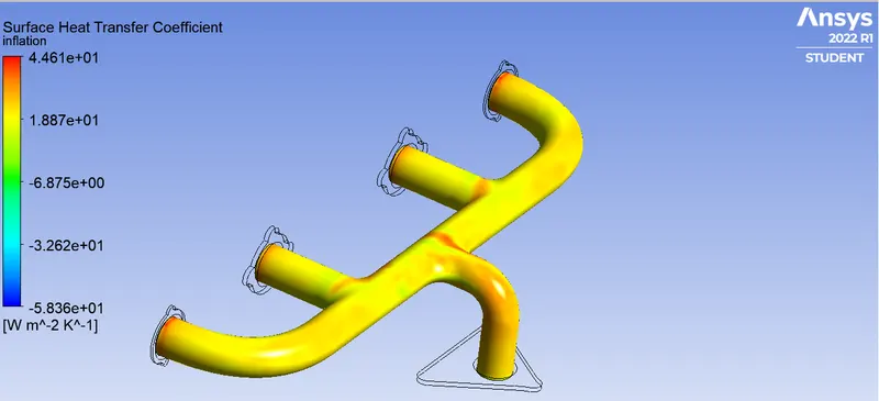
Max = 44.6141 `W/(m^2*k)`

Min = -58.3641 `W/(m^2*k)`

• k-omega model:

Temperature at cut-plane:

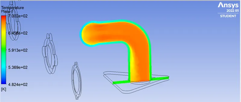
Max = 700.038 K

Min = 482.414 K

Velocity at cut-plane:

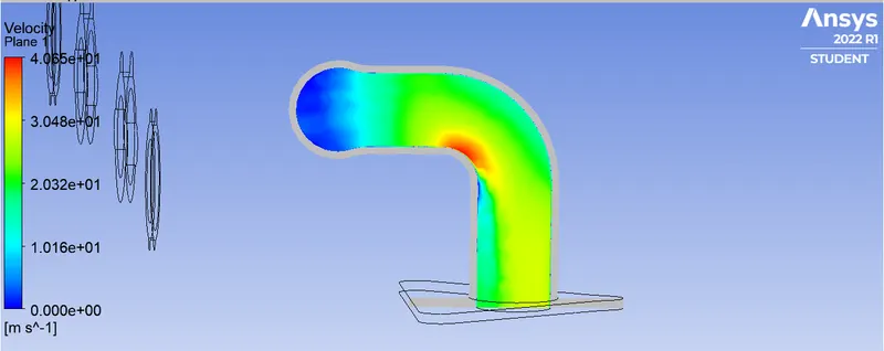
Max = 40.4645 m/s

Min = 0 m/s

Surface Heat Transfer coefficient:

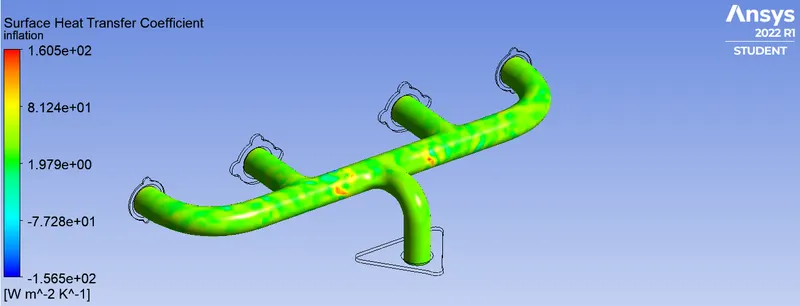
Max = 160.503 `W/(m^2*k)`

Min = -156.546 `W/(m^2*k)`

==============================================================================

Empiricle relations for Heat Transfer Coefficient:

• Generally for convection type problem, the HTC is analytically solved using Nusselt–Reynolds–Prandtl relations.

`Nu = C_(0)*Re^(C_(1))*Pr^(C_(2))*((mu_(blk))/(mu_(ski)))^(C_(3))`

• Then solve for 'h' in Nusselt Number equation.

`Nu = (h*l)/k`

Therefore, `h = (Nu*k)/l`

• The coefficients change with respect to geometry and are obtained by experimentation.

Reference: Link to paper

Conclusion: k-omega model resolves better results near the boundary and is effective in capturing the boundary layer phenomena.

==============================================================================