Week 4.1 - Genetic Algorithm
Problem Statement:
Try to understand the concept of genetic algorithm.
Q. Whats is genetic algorithm?
- The genetic algorithm is a method for solving both constrained and unconstrained optimization problems that is based on natural selection, the process that drives biological evolution.
- The genetic algorithm repeatedly modifies a population of individual solutions.
- At each step, the genetic algorithm selects individuals from the current population to be parents and uses them to produce the children for the next generation.
- Over successive generations, the population "evolves" toward an optimal solution.
- One can apply the genetic algorithm to solve a variety of optimization problems that are not well suited for standard optimization algorithms, including problems in which the objective function is discontinuous, nondifferentiable, stochastic, or highly nonlinear.
- The genetic algorithm can address problems of mixed integer programming, where some components are restricted to be integer-valued.
FLOW CHART:
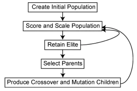
The genetic algorithm uses three main types of rules at each step to create the next generation from the current population:
-
Selection rules select the individuals, called parents, that contribute to the population at the next generation. The selection is generally stochastic, and can depend on the individuals' scores.
-
Crossover rules combine two parents to form children for the next generation.
-
Mutation rules apply random changes to individual parents to form children.
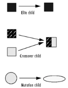
Reference link: Link
==============================================================================
Optimization problems:
In a genetic algorithm, a population of candidate solutions (called individuals, creatures, organisms, or phenotypes) to an optimization problem is evolved toward better solutions. Each candidate solution has a set of properties (its chromosomes or genotype) which can be mutated and altered; traditionally, solutions are represented in binary as strings of 0s and 1s, but other encodings are also possible.
The evolution usually starts from a population of randomly generated individuals, and is an iterative process, with the population in each iteration called a generation. In each generation, the fitness of every individual in the population is evaluated; the fitness is usually the value of the objective function in the optimization problem being solved. The more fit individuals are stochastically selected from the current population, and each individual's genome is modified (recombined and possibly randomly mutated) to form a new generation. The new generation of candidate solutions is then used in the next iteration of the algorithm. Commonly, the algorithm terminates when either a maximum number of generations has been produced, or a satisfactory fitness level has been reached for the population.
A typical genetic algorithm requires:
- a genetic representation of the solution domain,
- a fitness function to evaluate the solution domain.
A standard representation of each candidate solution is as an array of bits (also called bit set or bit string). Arrays of other types and structures can be used in essentially the same way. The main property that makes these genetic representations convenient is that their parts are easily aligned due to their fixed size, which facilitates simple crossover operations. Variable length representations may also be used, but crossover implementation is more complex in this case. Tree-like representations are explored in genetic programming and graph-form representations are explored in evolutionary programming; a mix of both linear chromosomes and trees is explored in gene expression programming.
Once the genetic representation and the fitness function are defined, a GA proceeds to initialize a population of solutions and then to improve it through repetitive application of the mutation, crossover, inversion and selection operators.
Reference link: link
==============================================================================
Code and Explanation:
CODE:
Function Code:
function f = stalagmite(input_vector)
    x = input_vector(1);
    y = input_vector(2);

    % Calculation
    f1 = (sin(5.1*pi*x+0.5))^6;
    f2 = (sin(5.1*pi*y+0.5))^6;
    f3 = exp((-4*log(2)*((x-0.0667)^2/0.64)));
    f4 = exp((-4*log(2)*((y-0.0667)^2/0.64)));

    f = -(f1*f2*f3*f4);
end
Main Code:
% Defining search space
x = linspace(0,0.6,150);
y = linspace(0,0.6,150);

% Creating 2D array
[xx yy] = meshgrid(x,y);  % creating a 2D array from row vector

% Evaluating the stalagmite function
for i = 1:length(xx)
   for j = 1:length(yy)
      input_vector(1) = xx(i,j);  % Making input_vector a row vector with two columns
      input_vector(2) = yy(i,j);
      f(i,j) = stalagmite(input_vector);
   end
end

% surfc(xx,yy,f);
% xlabel('x-axis')
% ylabel('y-axis')
% shading interp

% Study 1 - Unbounded Condition
num = 50;
tic
for i= 1:num
 [inputs, fopt(i)] = ga(@stalagmite,2);  % inputs will generate points where value of fval is minimum since ga gives minimum value.
 xopt(i) = inputs(1);
 yopt(i) = inputs(2);
end
study_time1 = toc;

% Plotting
figure(1)
subplot(2,1,1)
surfc(x,y,-f)
xlabel('x-axis')
ylabel('y-axis')
shading interp
hold on
plot3(xopt,yopt,-fopt,'marker','o','markersize',2,'markerfacecolor','r')
subplot(2,1,2)
plot(-fopt)
xlabel('Iterations')
ylabel('Function Minimum')


% Study 2 - Bounded Condition
tic
for i= 1:num
 [inputs, fopt(i)] = ga(@stalagmite,2,[],[],[],[],[0;0],[1;1]);  % inputs will generate points where value of fval is minimum since ga gives minimum value.
 xopt(i) = inputs(1);
 yopt(i) = inputs(2);
end
study_time2 = toc

% Plotting
figure(2)
subplot(2,1,1)
surfc(x,y,-f)
xlabel('x-axis')
ylabel('y-axis')
shading interp
hold on
plot3(xopt,yopt,-fopt,'marker','o','markersize',2,'markerfacecolor','r')
subplot(2,1,2)
plot(-fopt)
xlabel('Iterations')
ylabel('Function Minimum')

% Study 3
options = optimoptions('ga');
options = optimoptions(options,'PopulationSize',500);
tic
for i= 1:num
 [inputs, fopt(i)] = ga(@stalagmite,2,[],[],[],[],[0;0],[1;1],[],[],options);  % inputs will generate points where value of fval is minimum since ga gives minimum value.
 xopt(i) = inputs(1);
 yopt(i) = inputs(2);
end
study_time3 = toc

% Plotting
figure(3)
subplot(2,1,1)
surfc(x,y,-f)
xlabel('x-axis')
ylabel('y-axis')
shading interp
hold on
plot3(xopt,yopt,-fopt,'marker','o','markersize',2,'markerfacecolor','r')
subplot(2,1,2)
plot(-fopt)
xlabel('Iterations')
ylabel('Function Minimum')
Explanation:
- Two 1D arrays are created and then converted to 2D array which form the search space.
- An input_vector variable is declared to store the values and hence is an row vector with two columns.
- This is considered as an input to the stalagmite function which is calculated in its function code.
The function formulae:
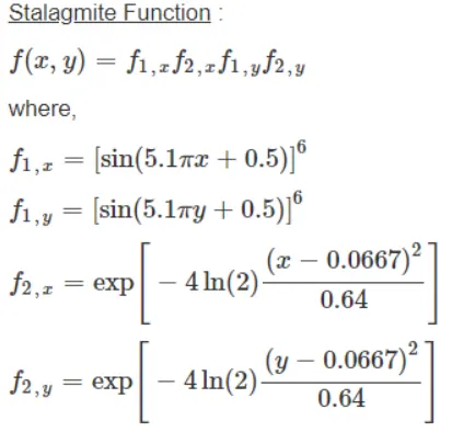
- The output by the stalagmite function are stored in a variable 'f'.
- Three different case studies are performed to give the maximum output.
- This is because the 'ga' function does not know the search space. (we know the search space as discribed above but the ga function does not know).
- In case study 1, the search space is random for the ga function and can go below and beyond the values of 0 and 0.6.
- [inputs,fopt], this basically gives out the maximum value of fopt a given point. And these points are stored seperately in xopt and yopt.
- Then we plot the graphs of the random points, the stalagmite and the function fopt vs iterations.
- 'surfc' is a command used to plot the surface graph in 3D and shading interp removes the mesh line from the graph.
- plot3 command is used to plot the 3D behaviour of a function.
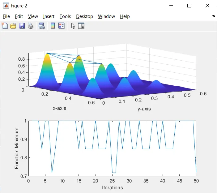
- Study 2 is similar to that of study 1 except the major change is, we have assigned the lower and upper bounds so that the values are well contained within the bounds.
- Inside the bracket, [] means that we are saying that there is no linear constraints in the function and hence at the end of the bracket we say that our lower and upper bounds are [0;0] [1;1].
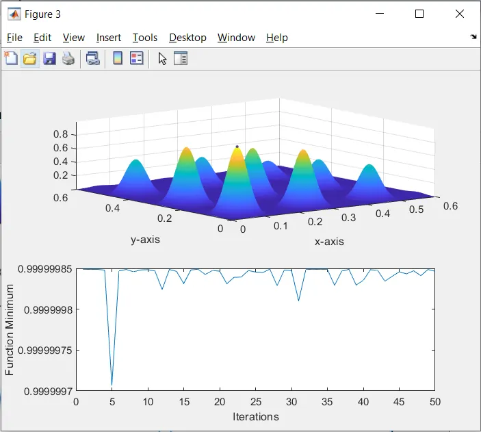
- In case study 3, after we specify the lower and upper bounds inside the bracket, we say that there are no nonlinear constraints and integer constrains in the function and is defined by [],[] inside the bracket.
- Finally the population size is defined using the options variable.
==============================================================================
Errors and rectification:

There is a typo. The spelling should be length not lenght.
==============================================================================
Results:
Study 1:
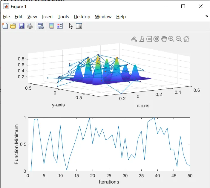
Study 2:
Study 3:
Conclusion:
- Study 1 gives new values every time we run it again.
- Study 2 bounds the solution within the the limits and takes a bit more time than Study 1.
- Study 3 gives the maximum value in the search space and take much more time when compared to other studies.