Week 1: Channel flow simulation using CONVERGE CFD
Aim: To carry out a channel flow simulation using CONVERGE.
Take away:
By the end of this article, one will be able to,
- Create a simple geometry of channel.
- Setup an entire case.
- Export all the input files required to run a simulation.
- Post process the data using PARAVIEW.
- Plot line data in CONVERGE Line plotting tab.
==============================================================================
Geometry:
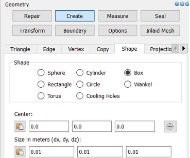
- Select "Create" >> "Shape" >> "Box".
- Center = 0.05, 0.0, 0.0
- "Size in meters tab" = 0.1, 0.01, 0.01 (Distance in x, y, z direction)
- Hit the create option.
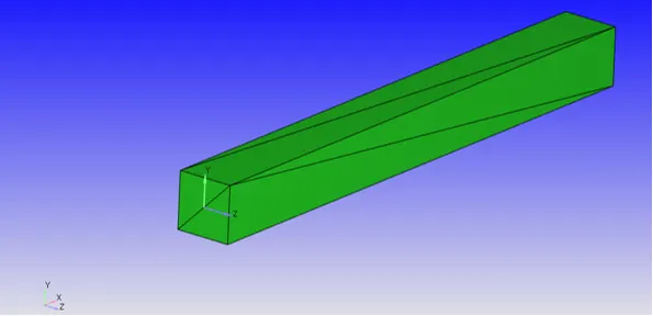
- One should get such a geometry.
==============================================================================
Assigning Boundary:
- Select the triangle tab.
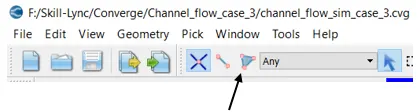
- In CONVERGE the geometry is divided into trigular faces/surfaces. In order to select the those triangle, the above highlighted tab should be enabled.
- It is important to assign boundaries to the geometry so the information can travel from one end to the other depending on the boundary condition applied.
- Select boundary tab.
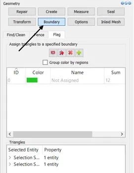
- Click on "Add" icon to include number of boundaries to be flagged.
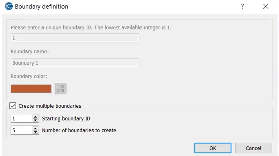
- Select "Create multiple boundaries" option to create multiple boundaries with a single click.
- Next step is to select the triangle and assign the boundaries.
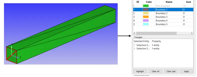
- Select the triangles, click on boundary 1 and apply.
- Select "Boundary 1", right click and rename it as inlet. Similar procedure must be followed for other boundary flagging.
==============================================================================
Case Setup:
- Select the "Begin Case Setup".
- Select Time-Based.
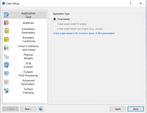
- Select "Materials".
- Predefined material: Air
- Deselect Reaction mechanism
- Select species.
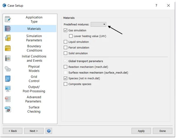
- Select "Physical Models" and deselect Turbulence modelling. It is a laminar flow problem.
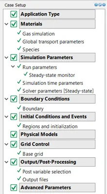
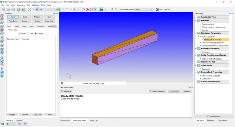
- Setting up a simulation is a step by step procedure. Which is followed as shown in the tree (above image).
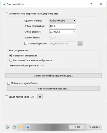
- Select "Gas simulation".
- No change. Set it with default values.
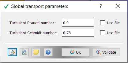
- Select "Global transport parameters". Set it to defalut values.
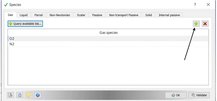
- Select "Species".
- Add O2 and N2.
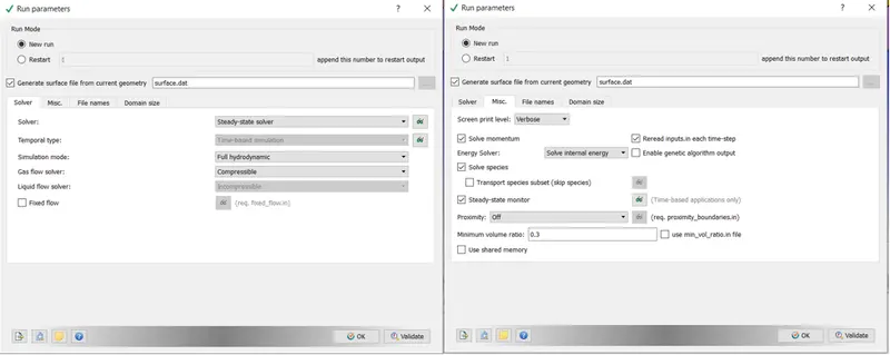
- Select "Run parameters".
- Make sure its steady-state, full hydrodynamics compressible and in "Misc" tab "Use shared memory" is unchecked.
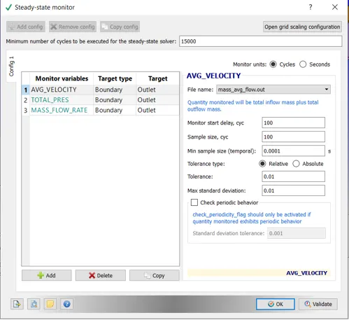
- Select "Steady-State monitors".
- Make sure "Monitor units" is in cycles when running a steady state simulation.
- "Minimum number of cycles to be executed for the steady-state solver: 15,000" = These many cycles will be executed irrespective of end cycle time and convergence.
- "Monitor start delay, cyc: 100" = It will start monitoring the variables after 100 cycles are completed.
- "Sample size, cyc: 100" = It will compare with the previous batch of 100 cycles in order to check convergence with the set tolerance value.
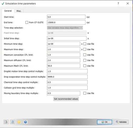
- Select "Simulation time parameters".
- Start time: 0
- End time: 15000
- Initial time step: 1e-09
- Minimum time step: 1e-09
- Maximum convection CFL limit: 1
- Keep others as default.
- Select "Solver parameters".
- Navier-Stokes solver type: Density-Based.
- Navigate to "Equations" tab and select "Pressure" and for "Preconditioners" select none.
- For "Maximum convection CFL limit (final stage)" assign a value of 0.5.
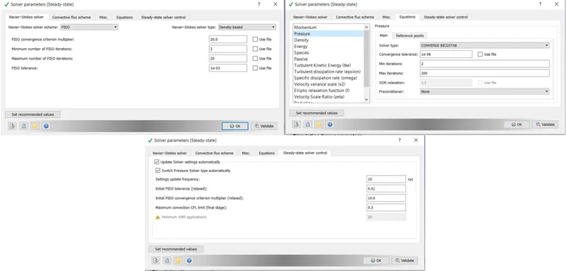
- Select "Boundary".
- Inlet:
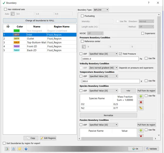
- Outlet:
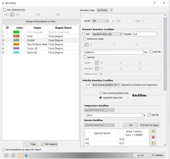
- Top-Bottom-Wall:
- Front 2D and Back 2D is assigned to let the software know that this is a 2D simulation.
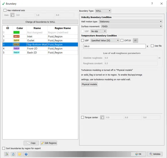
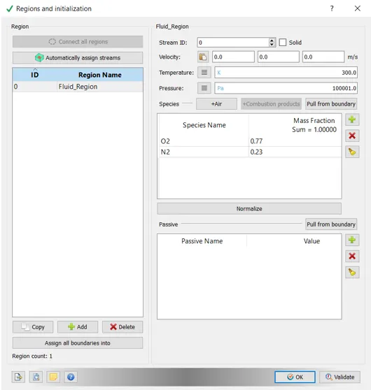
- Select "Regions and initialization".
- Create a "Region" , give it a name and rename it.
- Change the mass fraction of O2 and N2. (as shown in the figure)
- Make sure the pressure is same as the inlet pressure mentioned in the boundary tab.
==============================================================================
- Upto this point the setup is same for all the cases.
- Three cases have been discussed here:

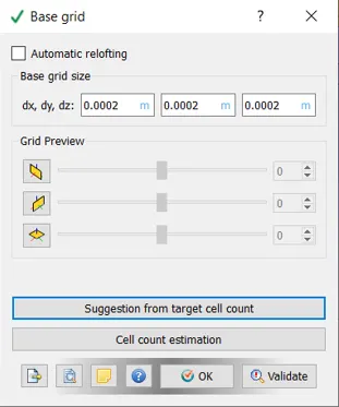
- Select "Base Grid".
- Input the above values for each new case created.
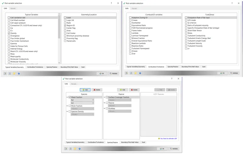
- Select "Post variable selection".
- Select the variable you want plot.
- Deselect all the turbulence parameters.
- Add species.
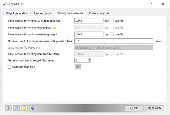
- Select "Output files".
- Time interval is set to 100.
==============================================================================
Results:
Case 1:
Results from CONVERGE:
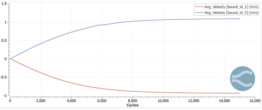
- Velocity Plot:
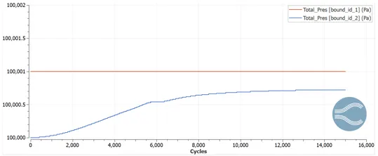
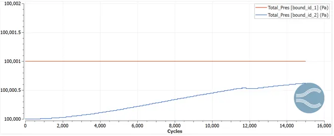
- Total Pressure Plot:
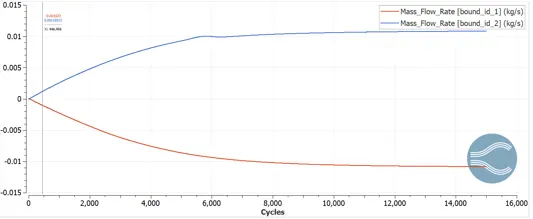
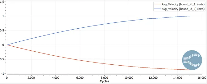
- Mass Flow Rate Plot:
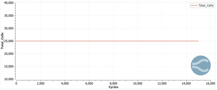
- Total Number of Cells:
Results from ParaView:
- Mesh:

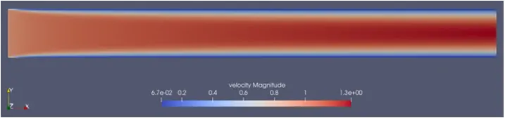
- Velocity Contour:
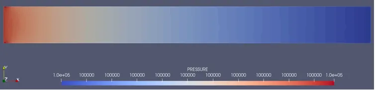
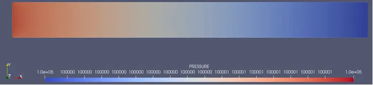
- Pressure Contour:
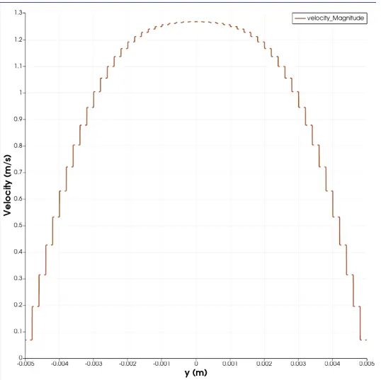
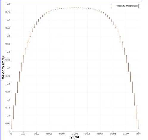
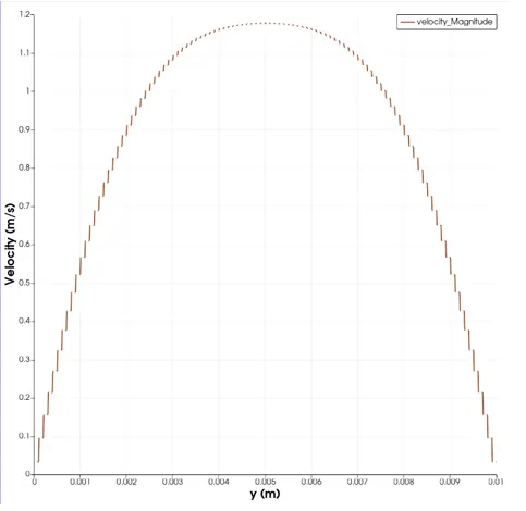
- Velocity Plot at x = 0.08m
Case 2:
Results from CONVERGE:
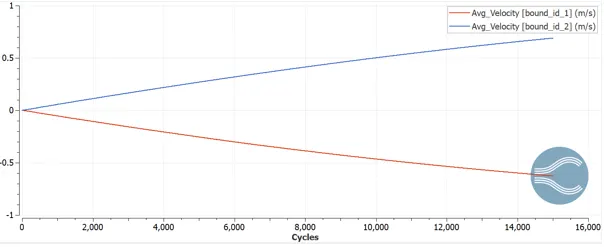
- Velocity Plot:
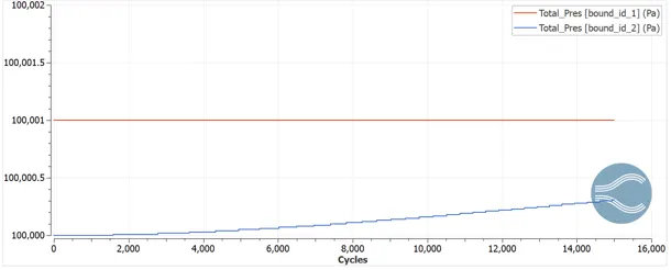
- Total Pressure Plot:
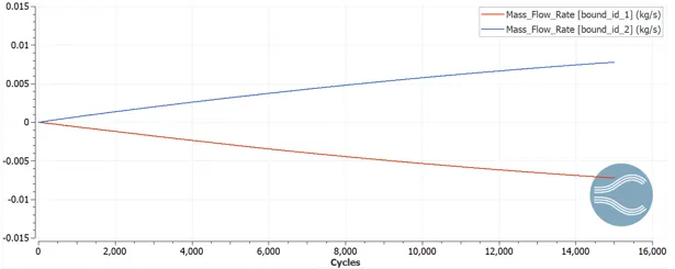
- Mass Flow Rate Plot:
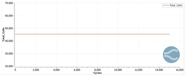
- Total Number of Cells:
Results from PARAVIEW:
- Mesh:

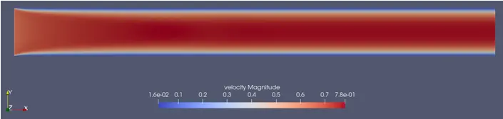
- Velocity Contour:
- Pressure Contour:
- Velocity Plot at x = 0.08m
Case 3:
Results from CONVERGE:
- Velocity Plot:
- Total Pressure Plot:
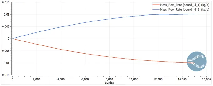
- Mass Flow Rate Plot:
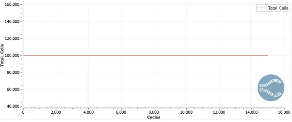
- Total Number of Cells:
Results from PARAVIEW:
- Mesh:

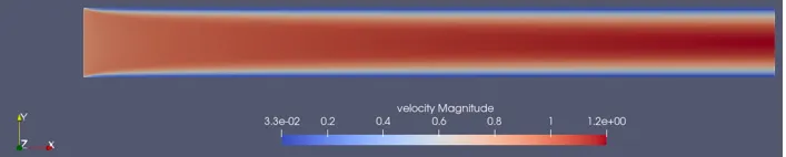
- Velocity Contour:
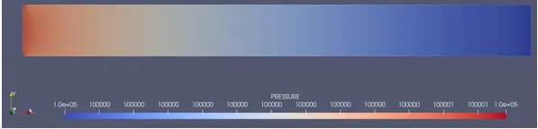
- Pressure Contour:
- Velocity Plot at x = 0.08m
==============================================================================
Animation:
- Case 1:
- Case 2:
- Case 3:
==============================================================================
Conclusion:
- It is necessary to run the simulation upto a point where it washes out the initial conditions and arrives at a steady solution.
- Mesh element size is important as the Navier-Stokes equations are solved at the cell centroid and have linear relation between ecah other.
- Near the wall, velocity profile is not linear and hence to capture the curvature profile of velocity, one needs to have a finner mesh near the wall.
- A point is arrived when there is no change in solution with furthur refinement of the grid. This is know as grid independence.
- In our problem, the 3rd case gives a smoother prfile when compared to the other two cases.