Week 3 - Solving second order ODEs

Problem Statement:

Use ode45 function to solve second order differential equation and simulate transient behaviour of a simple pendulem.

Formula:

`(d^2theta)/dt^2 + (b/m)((d theta)/dt) + (g/L)sin(theta) = 0`

g = gravity in m/s2,

L = length of the pendulum in m,

m = mass of the ball in kg,

b=damping coefficient.

Consideration,

L=1 metre,

m=1 kg,

b=0.05.

g=9.81 m/s2.

Main Code:

% To write a function to solve second order ODE

b = 0.05;  % Damping coefficient
g = 9.81;  % Acceleration due to gravity 
l = 1;     % Length of the string
m = 0.1;   % Mass of the system

% Inital Condition
theta_0 = [0;3];  % Initial condition for Angular displacement and Angular Velocity

% Time Points
t_span = linspace(0,20,500);  % Iteration time

% Solve ODE
[t, results] = ode45(@(t,theta) ode_func(t, theta, b,g,l,m), t_span, theta_0);

% Plotting
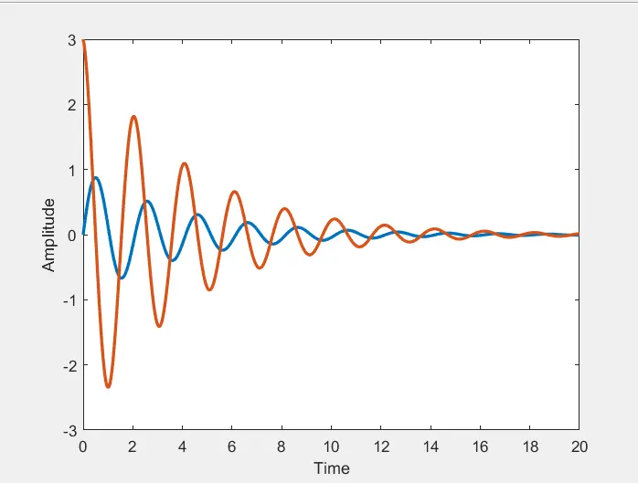
plot(t,results(:,1),'linewidth',2)
hold on
plot(t,results(:,2),'linewidth',2)
xlabel('Time')
ylabel('Amplitude')

% Animation
counter = 1;
theta1 = results(:,1);   % Taking all the values of all the rows of 1st column

for i = 1:length(results(:,1))
   % Starting Point
   x_start = 0;
   y_start = 0;
   theta2 = theta1(i);
   
   % End Point
   x_end = -l*sin(theta2);
   y_end = -l*cos(theta2);
   
   
   % Plotting
   figure(2)
   % Base of the pendulum 
   plot([-1,1],[0,0],'linewidth',2,'color','g')
   hold on
   % String of pendulum
   plot([x_start x_end],[y_start y_end],'linewidth',2,'color','b')
   hold on
   % Bob of prndulum
   plot(x_end, y_end, 'marker','o','linewidth',2,'markersize',30,'markerfacecolor','r')
   axis([-1.5 1.5 -1.5 0.15])
   hold off
   pause(0.03)
   M(counter) = getframe(gcf);
   counter = counter + 1;
end

% Creating a movie
movie(M)
videofile = VideoWriter('Simple_Pendulum.avi','Uncompressed AVI');
open(videofile);
writeVideo(videofile,M);
close(videofile);

Function Code:

function [dtheta_dt] = ode_func(t,theta,b,g,l,m)
    theta1 = theta(1);
    theta2 = theta(2);
    dtheta1_dt = theta2;
    dtheta2_dt = -(b/m)*theta2 -(g/l)*sin(theta1);
    dtheta_dt = [dtheta1_dt;dtheta2_dt];
end

Explanation:

• Every second order differential equation is brought down to first order differential equation.
• In this example, we say,

`theta = theta_1`

and,

`(d theta)/dt = (d theta_1)/dt = theta_2`

Therefore on simplifying the equation,

`(d theta_2)/dt + (b/m) theta_2 + (g/L) sin(theta_1)`

In matrix form,

Two equations have been created,

1) `(d theta_1)/dt = theta_2`

2)`(d theta_2)/dt = -(b/m) theta_2 - (g/L) sin(theta_1)`

• Initially the constant parameters are defined which do not change with respect to time and physically represent the dimensions of the system.
• theta_0 = [0;3] represent the intial conditions of the angular displacement (0) and angular velocity (3).
• t_span is the time iteration steps for iterative process done by ode45.
• The results are stored in 'results' variable.
• Inside ode45 command, the first parameter defines the dependent and independent variables for calculation.
• The following term is the function 'ode_func' which calculates `(d theta_1)/dt` and `(d theta_2)/dt`.
• ode45 function must know what are the initial conditions to solve the problem, therefore, the last two terms inside the ode45 function depicts the initial condition.
• The output is in the form of two column vectors, 1st is angular displacement and the 2nd is angular velocity.
• For animatoin, a counter variable is set to increment and stitch the frames.
• All the values of column (angular velocity) are stored in a variable theta1.
• A for loop is used to loop all the values from start to end.
• theta2 stores the values for looping the frames and is used to define the start and end point of the string for each change in value of i.
• To create a movie in MATLAB, MATLAB provides the following syntax:

movie(M)
videofile = VideoWriter('Simple_Pendulum.avi','Uncompressed AVI');
open(videofile);
writeVideo(videofile,M);
close(videofile);

• M is defined inside the for loop to access all the values of column 1 and form movie frame using 'getframe(gcf)' command.
• Finally the video/animation is written and stored inside respective folder.

Output: