Week 7 - Auto ignition using Cantera

Objective:

The aim is to simulate auto ignition using cantera for the fuel(methane) as per the given conditions.

Auto ignition temperature:

The auto ignition temperature or kindling point of a substance is the lowest temperature in which it spontaneously ignites in a normal atmosphere without an external source of ignition, such as a flame or spark. This temperature is required to supply the activation energy needed for combustion.

Ignition Delay:

Ignition delay time (IDT) is the time needed for a mixture of fuel and oxidizer to react at a certain temperature and pressure. This delay time is an important parameter for the engine designer and is typically determined experimentally.

Reactors and Reactor Networks:

Reactors:

A Cantera Reactor() represents the simplest form of a chemically reacting system. It corresponds to an extensive thermodynamic control volume VV, in which all state variables are homogeneously distributed. The system is generally unsteady -- that is, all states are functions of time. In particular, transient state changes due to chemical reactions are possible. However, thermodynamic (but not chemical) equilibrium is assumed to be present throughout the reactor at all instants of time.

Reactors can interact with the surrounding environment in multiple ways:

Expansion/compression work: By moving the walls of the reactor, its volume can be changed and expansion or compression work can be done by or on the reactor.

Heat transfer: An arbitrary heat transfer rate can be defined to cross the boundaries of the reactor.

Mass transfer: The reactor can have multiple inlets and outlets. For the inlets, arbitrary states can be defined. Fluid with the current state of the reactor exits the reactor at the outlets.

Surface interaction: One or multiple walls can influence the chemical reactions in the reactor. This is not just restricted to catalytic reactions, but mass transfer between the surface and the fluid can also be modelled.

All of these interactions do not have to be constant, but can vary as a function of time or state. For example, heat transfer can be described as a function of the temperature difference between the reactor and the environment, or the wall movement can be modelled depending on the pressure difference. Interactions of the reactor with the environment are defined on one or more walls, inlets and outlets.

In addition to single reactors, Cantera is also able to interconnect reactors into a Reactor Network. Each reactor in a network may be connected so that the contents of one reactor flow into another. Reactors may also be in contact with one another or the environment via walls that conduct heat or move to do work.

Code logic:

• Import and set the necessary libraries and plotting stuffs default.
• The instance object “gas” is created from the solution class.
• Define the reactor object “r” from the Ideal gas reactor class by passing gas object in it.
• Define the reactor network “sim” from the reactor net class by passing the reactor “r” in it.
• Similarly define the “states” from the solution array class by passing the gas object in it.
• Within the time loop, “advance” command is used for the purpose of advancing the reaction with time.
• Finally, append the necessary object and plot the result.

Code:

Part 1:

Case 1:

import numpy as np
import matplotlib.pyplot as plt
import cantera as ct
import sys

gas = ct.Solution('gri30.xml')
T = 1250
P = np.linspace(1,5,9)
t_start = 0.0
t_end = 10.0
dt = 1e-3
n = int((t_end - t_start)/dt)

'''
def float_range(t_start,t_end,dt):
	while t_end>t_start:
		yield t_start
		t_start += dt
'''

t_aigp = []
states1 = []

for i in P:
	gas.TPX = T,i*101325,{'CH4':1, 'O2':2, 'N2':7.52}
	T_aig = 0
	t_aig = 0
	r = ct.IdealGasReactor(gas)
	sim = ct.ReactorNet([r])
	time = 0.0
	states = ct.SolutionArray(gas, extra = ['time_in_ms','t'])
	print('{:10s} {:10s} {:10s}'.format('t[s]','T[K]','P[Pa]'))

	for j in range(n):
		time += 1e-3
		sim.advance(time)
		states.append(r.thermo.state,time_in_ms = time*1e3,t = time)
		print('{:10.3e} {:10.3f} {:10.3f}'.format(sim.time,r.T,r.thermo.P))
	
	states1.append(states.T)

	for j in range(n):
		error = states.T[j] - T - 400

		if error > 0:
			T_aig = states.T[j]
			t_aig = states.time_in_ms[j]
			break
	
	t_aigp.append(t_aig)

states1 = np.array(states1)

for k in range(len(P)):
	plt.figure(1)
	plt.plot(states1[k])
	plt.xlabel('Number of time steps')
	plt.ylabel('Temperature')
	plt.title('Auto ignition Temperature by varying pressure')
	plt.legend(['1 bar','1.5 bar','2 bar', '2.5 bar', '3 bar', '3.5 bar', '4 bar', '4.5 bar', '5 bar'])

plt.figure(2)
plt.plot(P,t_aigp,'-o')
plt.xlabel('Presure')
plt.ylabel('Auto ignition time in ms')
plt.title('Ignition delay vs Presure')
plt.show()

Result:

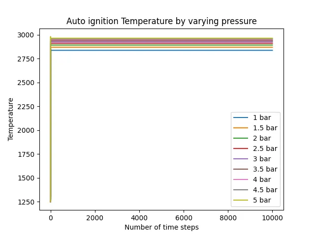
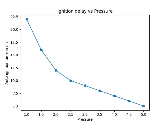
From the obtained result, ignition delays when pressure is low. When it starts to increase gradually, ignition delay time also starts to decrease.

Case 2:

import numpy as np
import matplotlib.pyplot as plt
import cantera as ct
import sys

gas = ct.Solution('gri30.xml')
P = 5*101325
T = np.linspace(950,1450,11)
t_start = 0.0
t_end = 10.0
dt = 1e-3
n = int((t_end - t_start)/dt)
'''
def float_range(t_start,t_end,dt):
	while t_end>t_start:
		yield t_start
		t_start += dt
'''

t_aigt = []
states1 = []

for i in T:
	gas.TPX = i,P,{'CH4':1, 'O2':2, 'N2':7.52}
	T_aig = 0
	t_aig = 0
	r = ct.IdealGasReactor(gas)
	sim = ct.ReactorNet([r])
	time = 0.0
	states = ct.SolutionArray(gas, extra = ['time_in_ms','t'])
	print('{:10s} {:10s} {:10s}'.format('t[s]','T[K]','P[Pa]'))

	for j in range(n):
		time += 1e-3
		sim.advance(time)
		states.append(r.thermo.state,time_in_ms = time*1e3,t = time)
		print('{:10.3e} {:10.3f} {:10.3f}'.format(sim.time,r.T,r.thermo.P))
	
	states1.append(states.T)

	for j in range(n):
		error = states.T[j] - i - 400

		if error > 0:
			T_aig = states.T[j]
			t_aig = states.time_in_ms[j]
			break
	
	t_aigt.append(t_aig)

states1 = np.array(states1)

for k in range(len(T)):
	plt.figure(1)
	plt.plot(states1[k])
	plt.xlabel('Number of time steps')
	plt.ylabel('Temperature')
	plt.title('Auto ignition Temperature by varying temperature')
	plt.legend(['950 K','1000 K','1050 K', '1100 K', '1150 K', '1200 K', '1250 K', '1300 K', '1350 K', '1400 K', '1450 K'])

plt.figure(2)
plt.plot(T,t_aigt,'-o')
plt.xlabel('Presure')
plt.ylabel('Auto ignition time in ms')
plt.title('Ignition delay vs Temperature')
plt.show()

Result:

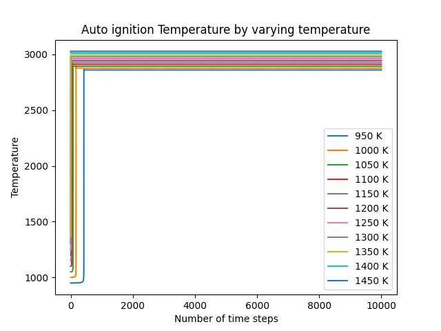
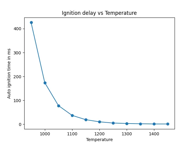
Similar result is obtained as of case 1. Ignition delays when temperature is low. When it starts to increase gradually, ignition delay time also starts to decrease.

Part 2:

Case 1:

import numpy as np
import matplotlib.pyplot as plt
import cantera as ct
import sys

gas = ct.Solution('gri30.xml')
P = 5*101325
T = 1000
t_start = 0.0
t_end = 10.0
dt = 1e-3
n = int((t_end - t_start)/dt)
'''
def float_range(t_start,t_end,dt):
	while t_end>t_start:
		yield t_start
		t_start += dt
'''

t_aigt = []
states1 = []

gas.TPX = T,P,{'CH4':1, 'O2':2, 'N2':7.52}
T_aig = 0
t_aig = 0
r = ct.IdealGasReactor(gas)
sim = ct.ReactorNet([r])
time = 0.0
states = ct.SolutionArray(gas, extra = ['time_in_ms','t'])
print('{:10s} {:10s} {:10s}'.format('t[s]','T[K]','P[Pa]'))

for j in range(n):
	time += 1e-3
	sim.advance(time)
	states.append(r.thermo.state,time_in_ms = time*1e3,t = time)
	print('{:10.3e} {:10.3f} {:10.3f}'.format(sim.time,r.T,r.thermo.P))
	
states1.append(states.T)

for j in range(n):
	error = states.T[j] - T - 400

	if error > 0:
		T_aig = states.T[j]
		t_aig = states.time_in_ms[j]
		break
	t_aigt.append(t_aig)

plt.figure(1)
plt.subplot(3,1,1)
plt.plot(states.t,states.X[:,gas.species_index('H2O')])
plt.xlabel('Time(ms)')
plt.ylabel('H2O mole fraction')
plt.title('Auto ignition Temperature by varying moler concentration')
plt.subplot(3,1,2)
plt.plot(states.t,states.X[:,gas.species_index('O2')])
plt.xlabel('Time(ms)')
plt.ylabel('O2 mole fraction')
plt.subplot(3,1,3)
plt.plot(states.t,states.X[:,gas.species_index('OH')])
plt.xlabel('Time(ms)')
plt.ylabel('OH mole fraction')
plt.show()

Result:

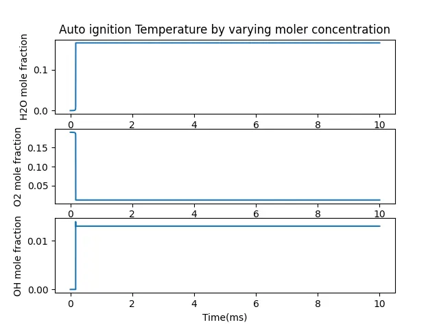
From the result obtained, each species results are varying when temperature and pressure is 1000K and 5 bar. H2O and OH concentration is increasing and O2 concentration is decreasing which means O2 is consumed during the combustion process and others are formed by the reaction.

Case 2:

import numpy as np
import matplotlib.pyplot as plt
import cantera as ct
import sys

gas = ct.Solution('gri30.xml')
T = 500
P = 5*101325
gas.TPX = T,P,{'CH4':1, 'O2':2, 'N2':7.52}
r = ct.IdealGasReactor(gas)
sim = ct.ReactorNet([r])
time = 0.0
states = ct.SolutionArray(gas)

for n in range(1000):
	time += 1e-3
	sim.advance(time)
	states.append(r.thermo.state)

plt.plot(states.T)
plt.xlabel('Number of time steps')
plt.ylabel('Temperature')
plt.title('Auto ignition when Temperature is 500 K')
plt.show()

Result:

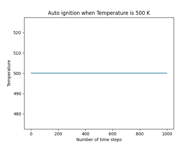
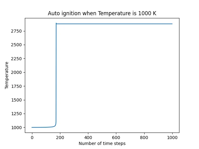
From the result obtained, When temperature is 500K, no sign of igniting combustion. When temperature is 1000K, ignition is initiated. When temperature is low, there is no possibilites of starting the combustion process. It should be at some range, then only the process can be initiate.