Week 6 - Multivariate Newton Rhapson Solver

Objective: The aim is to solve the solution for the given different non-linear system equation by using backward difference in the Newton Raphson solver.

The reason calling the given system of equations as non-linear is because of each one separately having an unknown variable.

The conditions to solve the solution is to estimate the Jacobian numerically not analytically.

At the start, employing the backward difference in the given equation. The general format is as follows

yⁿ = y^n-1 + dt*f(x)

Now, convert it in the form of RHS – LHS = 0

y^n-1 + dt*f(x) - yⁿ = 0

Here, yⁿ - New value

y^n-1 - Old value

dt - Time step

The way to estimate the Jacobian numerically in general follows the formula below

df/dy = (f(x+h) – f(x))/h

For finding the new value by using Newton Raphson solver, follow the following general formula

y_n+1 = y_n – α*(J^-1 * F)

To solve it for more species, we need to form the above equation into matrix form for the set of dimensions properly.

Now, simulation to be done for the given 10 minutes by using backward scheme in the implicit function for the outer time integration loop.

df/dy = (f(x) – f(x-h))/h

Code:

import numpy as np
from numpy.linalg import inv
import matplotlib.pyplot as plt

t_start = 0
t_end = 600
n = 1200
dt = (t_end - t_start)/(n)

# Initial comditions
y1 = 1
y2 = 0
y3 = 0

def f1(y1, y2, y3, dt, y1_old, y2_old, y3_old):

	return y1_old + dt*(-0.04*y1 + (y2*y3*pow(10,4))) - y1

def f2(y1, y2, y3, dt, y1_old, y2_old, y3_old):

	return y2_old + dt*(0.04*y1) - dt*(y2*y3*pow(10,4)) - dt*(3*pow(y2,2)*pow(10,7)) - y2

def f3(y1, y2, y3, dt, y1_old, y2_old, y3_old):

	return y3_old + dt*(3*pow(y2,2)*pow(10,7)) - y3

def jacobian(y1, y2, y3, dt, y1_old, y2_old, y3_old):

	# defining the jacobian

	J = np.ones((3,3))
	h = 1e-4

	# Row1
	J[0,0] = (f1(y1+h, y2, y3, dt, y1_old, y2_old, y3_old) - f1(y1, y2, y3, dt, y1_old, y2_old, y3_old))/h
	J[0,1] = (f1(y1, y2+h, y3, dt, y1_old, y2_old, y3_old) - f1(y1, y2, y3, dt, y1_old, y2_old, y3_old))/h
	J[0,2] = (f1(y1, y2, y3+h, dt, y1_old, y2_old, y3_old) - f1(y1, y2, y3, dt, y1_old, y2_old, y3_old))/h

	# Row2
	J[1,0] = (f2(y1+h, y2, y3, dt, y1_old, y2_old, y3_old) - f2(y1, y2, y3, dt, y1_old, y2_old, y3_old))/h
	J[1,1] = (f2(y1, y2+h, y3, dt, y1_old, y2_old, y3_old) - f2(y1, y2, y3, dt, y1_old, y2_old, y3_old))/h
	J[1,2] = (f2(y1, y2, y3+h, dt, y1_old, y2_old, y3_old) - f2(y1, y2, y3, dt, y1_old, y2_old, y3_old))/h

	# Row3
	J[2,0] = (f3(y1+h, y2, y3, dt, y1_old, y2_old, y3_old) - f3(y1, y2, y3, dt, y1_old, y2_old, y3_old))/h
	J[2,1] = (f3(y1, y2+h, y3, dt, y1_old, y2_old, y3_old) - f3(y1, y2, y3, dt, y1_old, y2_old, y3_old))/h
	J[2,2] = (f3(y1, y2, y3+h, dt, y1_old, y2_old, y3_old) - f3(y1, y2, y3, dt, y1_old, y2_old, y3_old))/h

	return J

# Newton Raphson
def newton_raphson(y1,y2,y3,y1_g,y2_g,y3_g,dt):
	
	# numpy column vector
	y_old = np.ones((3,1))
	y_old[0] = y1_g
	y_old[1] = y2_g
	y_old[2] = y3_g

	# numpy column vector for F
	F = np.copy(y_old)

	# properties for newton raphson solver
	alpha = 1
	tol = 1e-5

	# Initial error
	error = 9e9
	iter = 1

	while error > tol:

		J = jacobian(y_old[0],y_old[1],y_old[2],dt,y1,y2,y3)

		F[0] = f1(y_old[0],y_old[1],y_old[2],dt,y1,y2,y3)
		F[1] = f2(y_old[0],y_old[1],y_old[2],dt,y1,y2,y3)
		F[2] = f3(y_old[0],y_old[1],y_old[2],dt,y1,y2,y3)

		y_new = y_old - alpha*(np.matmul(inv(J), F))
		error = np.max(np.abs(y_new - y_old))

		y_old = y_new

		log_message = 'iteration # - {0} y1 {1} y2 {2} y3 {3}'.format(iter, y_new[0], y_new[1], y_new[2])
		print(log_message)
		iter = iter + 1

	return [y_new[0], y_new[1], y_new[2]]

def implicit(y1, y2, y3, t_start, t_end, dt):

	t = np.arange(t_start, t_end, dt)
	time = len(t)

	y_1 = np.zeros(time)
	y_2 = np.zeros(time)
	y_3 = np.zeros(time)

	y_1[0] = y1
	y_2[0] = y2
	y_3[0] = y3

	y1_g = 0
	y2_g = 0
	y3_g = 0

	for i in range (1,time):

		y_1[i], y_2[i], y_3[i] = newton_raphson(y_1[i-1],y_2[i-1],y_3[i-1],y1_g,y2_g,y3_g,dt)

		y1_g = y_1[i]
		y2_g = y_2[i]
		y3_g = y_3[i]

	return [t,y_1,y_2,y_3]
	

t, y1, y2, y3 = implicit(1, 0, 0, 0, 600, 0.1)

plt.plot(t,y1)
plt.plot(t,y2)
plt.plot(t,y3)
plt.xlabel('Simulation time')
plt.ylabel('Species Initial guess values')
plt.legend(['y1','y2','y3'])
plt.title('Multivariate Newton Raphson')
plt.show()

Code logic:

1. Initially, starts with importing the necessary library to solve the solution.
2. Next, defining the function for the given system of equation by converting into a specific form and return it
3. Define the Jacobian function to return the variable in the matrix form by numerically.
4. Define the Newton Raphson function to return the new values of the species by updating old values.
5. Define the implicit function for the outer time loop integration by assembling ODE and run the Newton Raphson till the solution gets converge. Finally, get the new values with proper updates of the values and ends the time loop
6. Plot the graph for the simulation time and the various species.

Result:

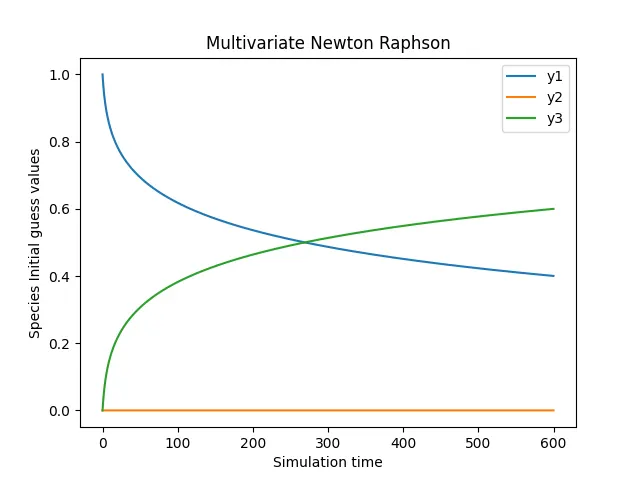
From the graph obtained, we can observe that when time starts to run, the values of each species from its guess values starts varying according to their system. Though the result of each species varies when time steps forward, the result is stable due to the implicit method. If we program the same thing in the explicit scheme by dependent of time step, it gives various results. When the time step is small, the result is in stable and vice versely unstable when the time step is large.