Week 3.5 - Deriving 4th order approximation of a 2nd order derivative using Taylor Table method

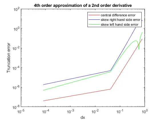
Objective: The aim is to evaluate the second-order derivative of the analytical function exp(x)*cos(x) and compare it with the 3 numerical approximations that you have derived.

Derivation for fourth order approximation of the second order derivative:

Central difference:

This method is nothing but gathering the information from the surrounding nodal points by having a node as its centre. The distance between each point is dx.

Here, I’m taking surrounding nodes as (i-2), (i-1), (i+1), (i+2) by having centre node as (i).

From considered information, the hypothesis equation is as follows

`(∂^2 u)/(∂x^2) = a f(i-2) + b f(i-1) + c f(i) + d f(i+1) + e f(i+2)`

Now, using Taylor’s method to find the coefficients. To do so, writing Taylor series approach for each term

`a f(i-2) = a f(i) - a f’(i)*2Δx + (a f’’(i)*(2Δx)2)/(2!) - (a f’’’(i)*(2Δx)3)/(3!) + (a f’’’’’(i)*(2Δx)4)/(4!) - (a f’’’’’’(i)*(2Δx)5)/(5!) + (a f’’’’’’’(i)*(2Δx)6)/(6!)`

`b f(i-1) = b f(i) - b f’(i)*Δx + (b f’’(i)*(Δx)^2)/(2!) - (b f’’’(i)*(Δx)^3)/(3!) + (b f’’’’’(i)*(Δx)^4)/(4!) - (b f’’’’’’(i)*(Δx)^5)/(5!) + (b f’’’’’’’(i)*(Δx)^6)/(6!)`

`c f(i) = c f(i)`

`d f(i+1) = d f(i) + d f’(i)*Δx + (d f’’(i)*(Δx)^2)/(2!) + (d f’’’(i)*(Δx)^3)/(3!) + (d f’’’’’(i)*(Δx)^4)/(4!) + (d f’’’’’’(i)*(Δx)^5)/(5!) + (d f’’’’’’’(i)*(Δx)^6)/(6!)`

`e f(i+2) = e f(i) + e f’(i)*2Δx + (e f’’(i)*(2Δx)^2)/(2!) + (e f’’’(i)*(2Δx)^3)/(3!) + (e f’’’’’(i)*(2Δx)^4)/(4!) + (e f’’’’’’(i)*(2Δx)^5)/(5!) + (e f’’’’’’’(i)*(2Δx)^6)/(6!)`

Taylor’s table for the above equation

	f(i)	f’(i)*Δx	f’’(i)*(Δx^2)	f’’’(i)*(Δx^3)	f’’’(i)*(Δx^4)	f’’’(i)*(Δx^5)	f’’’(i)*(Δx^6)
a f(i-2)	a	-2a	4a/2	-8a/6	16a/24	-32a/120	64a/240
b f(i-1)	b	-b	b/2	-b/6	b/24	-b/120	b/240
c f(i)	c	0	0	0	0	0	0
d f(i+1)	d	d	d/2	d/6	d/24	d/120	d/240
e f(i+2)	e	2e	4e/2	8e/6	16e/24	32e/120	64e/240
Summation of hypothesis equation	0	0	1	0	0	?	?

Now, add all the columns to form as equation to find the coefficients. The summation of second order is 1 because of we are solving only for it. Other than this, everything is equal to 0.

a + b + c + d + e = 0

-2a - b + 0 - d + 2e = 0

2a + (b/2) + 0 + (d/2) + 2e = 1

(-8a/6) + (-b/6) + 0 + (d/6) + (8e/6) = 0

(16a/24) + (b/24) + 0 + (d/24) + (16e/24) = 0

Write the above equations in the matrix inversion method, AX = B

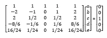
For find these coefficients, I used Matlab command window by storing values of A & B to get variable X values. The format I used is

X = inv(A)*B

Then, the output of the coefficients are

a = - 1/12

b = 4/3

c = - 5/2

d = 4/3

e = - 1/12

Now, divide the hypothesis equation by Δx²

^{`(∂^2 u)/(∂x^2) = (a*f(i-2) + b*f(i-1) + c*f(i) + d*f(i+1) + e*f(i+2))/(∆x)^2`}

Apply the coefficients to get the fourth order approximation

`(∂^2 u)/(∂x^2) = ((-1/12)*f(i-2) +(4/3)*f(i-1) +(-5/2)*f(i) +(4/3)*f(i+1) +(-1/12)*f(i+2))/(∆x^2)`

From Taylor’s table, to know the unknown of the summation for the fifth & sixth order derivative write the equation by adding the values of the table of its own derivative as coefficient.

`(∂^2 u)/(∂x^2)` = (a + b + c + d + e) f(i) + (-2a - b + 0 - d + 2e) f’(i) Δx + (2a + (b/2) + 0 + (d/2) + 2e) f’’(i) Δx² + ((-8a/6) + (-b/6) + 0 + (d/6) + (8e/6)) f’’’(i) Δx³ + ((16a/24) + (b/24) + 0 + (d/24) + (16e/24)) f’’’(i) Δx⁴ + ((-32a/120) + (-b/120) + 0 + (d/120) + (32e/120))f’’’’’(i) Δx⁵ + ((64a/240) + (b/240) + 0 + (d/240) + (64e/240))f’’’’’’(i) Δx⁶

Now, order of all is 0 except second derivative. In order to check it in in fifth & sixth, divide the above equation by Δx². Then, fifth one is become third derivative. When you see the equation of this coefficient, its equally stable by its sign and also coefficient value of a & e is equal. If, apply so then coefficient become zero & it will get neglect. The sixth order become Δ⁴. Here, Δ⁴ is the truncation error for the fourth order. The final equation is

`(∂^2 u)/(∂x^2)` = (2a + (b/2) + 0 + (d/2) + 2e) f’’(i) + ((64a/240) + (b/240) + 0 + (d/240) + (64e/240))f’’’’’’(i) Δx⁴

Skew right:

This method is nothing but gathering the information from the right side nodal points from its centre.

Here, I’m taking nodes of right side (i+1), (i+2), (i+3), (i+4), (i+5) from its centre node of (i).

From considered information, the hypothesis equation is as follows

`(∂^2 u)/(∂x^2)`= a f(i) + b f(i+1) + c f(i+2) + d f(i+3) + e f(i+4) + g f(i+5)

Now, using Taylor’s method to find the coefficients. To do so, writing Taylor series approach for each term

a f(i) = a f(i)

`b f(i+1) = b f(i) + b f’(i)*Δx + (b f’’(i)*(Δx)^2)/(2!) + (b f’’’(i)*(Δx)^3)/(3!) + (b f’’’’’(i)*(Δx)^4)/(4!) + (b f’’’’’’(i)*(Δx)^5)/(5!) + (b f’’’’’’’(i)*(Δx)^6)/(6!)`

`c f(i+2) = c f(i) + c f’(i)*2Δx + (c f’’(i)*(2Δx)^2)/(2!) + (c f’’’(i)*(2Δx)^3)/(3!) + (c f’’’’’(i)*(2Δx)^4)/(4!) + (c f’’’’’’(i)*(2Δx)^5)/(5!) + (c f’’’’’’’(i)*(2Δx)^6)/(6!)`

`d f(i+3) = d f(i) + d f’(i)*3Δx + (d f’’(i)*(3Δx)^2)/(2!) + (d f’’’(i)*(3Δx)^3)/(3!) + (d f’’’’’(i)*(3Δx)^4)/(4!) + (d f’’’’’’(i)*(3Δx)^5)/(5!) + (d f’’’’’’’(i)*(3Δx)^6)/(6!)`

`e f(i+4) = e f(i) + e f’(i)*4Δx + (e f’’(i)*(4Δx)^2)/(2!) + (e f’’’(i)*(4Δx)^3)/(3!) + (e f’’’’’(i)*(4Δx)^4)/(4!) + (e f’’’’’’(i)*(4Δx)^5)/(5!) + (e f’’’’’’’(i)*(4Δx)^6)/(6!)`

`g f(i+5) = g f(i) + g f’(i)*5Δx + (g f’’(i)*(5Δx)^2)/(2!) + (g f’’’(i)*(5Δx)^3)/(3!) + (g f’’’’’(i)*(5Δx)^4)/(4!) + (g f’’’’’’(i)*(5Δx)^5)/(5!) + (g f’’’’’’’(i)*(5Δx)^6)/(6!)`

Taylor’s table for the above equation

	f(i)	f’(i)*Δx	f’’(i)*(Δx^2)	f’’’(i)*(Δx^3)	f’’’(i)*(Δx^4)	f’’’(i)*(Δx^5)	f’’’(i)*(Δx^6)
a f(i)	a	0	0	0	0	0	0
b f(i+1)	b	b	b/2	b/6	b/24	b/120	b/720
c f(i+2)	c	2c	4c/2	8c/6	16c/24	32c/120	64c/720
d f(i+3)	d	3d	9d/2	27d/6	81d/24	243d/120	729d/720
e f(i+4)	e	4e	16e/2	64e/6	256e/24	1024e/120	5096e/720
g f(i+5)	g	5g	25g/2	125g/6	652g/24	3125g/120	15625g/720
Summation of hypothesis equation	0	0	1	0	0	0	?

Now, add all the columns to form as equation to find the coefficients. The summation of second order is 1 because of we are solving only for it. Other than this, everything is equal to 0.

a + b + c + d + e + g = 0

0 + b + 2c + 3d + 4e + 5g = 0

0 + (b/2) + (4c/2) + (9d/2) + (16e/2) + (25g/2) = 1

0 + (b/6) + (8c/6) + (27d/6) + (64e/6) + (125g/6) = 0

0 + (b/24) + (16c/24) + (81d/24) + (256e/24) + (625g/24) = 0

0 + (b/120) + (32c/120) + (243d/120) + (1024e/120) + (3125g/120) = 0

Write the above equations in the matrix inversion method, AX = B

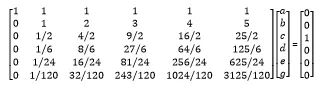
For find these coefficients, I used Matlab command window by storing values of A & B to get variable X values. The format I used is

X = inv(A)*B

Then, the output of the coefficients are

a = 15/4

b = (-77/6)

c = (107/6)

d = -13

e = 61/12

g = (-5/6)

Now, divide the hypothesis equation by Δx²

^{`(∂^2 u)/(∂x^2) = (a f(i) + b f(i+1) + c f(i+2) + d f(i+3) + e f(i+4) + g f(i+5))/(∆x^2)`}

Apply the coefficients to get the fourth order approximation

`(∂^2 u)/(∂x^2) = ((15/4) f(i) +(-77/6) f(i+1) +(107/6) f(i+2) +(-13) f(i+3) +(61/12) f(i+4) +(-5/6) f(i+5))/(∆x^2)`

From Taylor’s table, to know the unknown of the summation for the fifth & sixth order derivative write the equation by adding the values of the table of its own derivative as coefficient.

`(∂^2 u)/(∂x^2)` = (a + b + c + d + e + g) f(i) + (b + 2c + 3d + 4e + 5g) f’(i)Δx + ((b/2) + 2c + (9d/2) + (16e/2) + (25g/2)) f’’(i) Δx² + ((b/6) + (8c/6) + (27d/6) + (64e/6) + (125g/6)) f’’’(i) Δx³ + ((b/24) + (16c/24) + (81d/24) + (256e/24) + (625g/24)) f’’’(i) Δx⁴ + ((b/120) + (32c/120) + (243d/120) + (1024e/120) + (3125g/120))f’’’’’(i) Δx⁵ + ((64c/720) + (b/720) + (729d/720) + (5096e/720) + (15625g/720))f’’’’’’(i) Δx⁶

Now, order of all is 0 except second derivative. In order to check it in in fifth & sixth, divide the above equation by Δx². Then, fifth one is become third derivative. So, the order of Δ³ is 0 as per known. It will get neglect. The sixth order become Δ⁴. Here, Δ⁴ is the truncation error for the fourth order. The final equation is

`(∂^2 u)/(∂x^2)` = ((b/2) + 2c + (9d/2) + (16e/2) + (25g/2)) f’’(i) + ((64c/720) + (b/720) + (729d/720) + (5096e/720) + (15625g/720))f’’’’’’(i) Δx⁴

Skew left:

This method is nothing but gathering the information from the left side nodal points from its centre.

Here, I’m taking nodes of left side (i-5), (i-4), (i-3), (i-2), (i-1) from its centre node of (i).

From considered information, the hypothesis equation is as follows

= a f(i-5) + b f(i-4) + c f(i-3) + d f(i-2) + e f(i-1) + g f(i)

Now, using Taylor’s method to find the coefficients. To do so, writing Taylor series approach for each term

`a f(i-5) = a f(i) - a f’(i)*5Δx + (a f’’(i)*(5Δx)^2)/(2!) - (a f’’’(i)*(5Δx)^3)/(3!) + (a f’’’’’(i)*(5Δx)^4)/(4!) - (a f’’’’’’(i)*(5Δx)^5)/(5!) + (a f’’’’’’’(i)*(5Δx)^6)/(6!)`

`b f(i-4) = b f(i) - b f’(i)*4Δx + (b f’’(i)*(4Δx)^2)/(2!) - (b f’’’(i)*(4Δx)^3)/(3!) + (b f’’’’’(i)*(4Δx)^4)/(4!) - (b f’’’’’’(i)*(4Δx)^5)/(5!) + (b f’’’’’’’(i)*(4Δx)^6)/(6!)`

`c f(i-3) = c f(i) - c f’(i)*3Δx + (c f’’(i)*(3Δx)^2)/(2!) - (c f’’’(i)*(3Δx)^3)/(3!) + (c f’’’’’(i)*(3Δx)^4)/(4!) - (c f’’’’’’(i)*(3Δx)^5)/(5!) + (c f’’’’’’’(i)*(3Δx)^6)/(6!)`

`d f(i-2) = d f(i) - d f’(i)*2Δx + (d f’’(i)*(2Δx)^2)/(2!) - (d f’’’(i)*(2Δx)^3)/(3!) + (d f’’’’’(i)*(2Δx)^4)/(4!) - (d f’’’’’’(i)*(2Δx)^5)/(5!) + (d f’’’’’’’(i)*(2Δx)^6)/(6!)`

`e f(i-1) = e f(i) - e f’(i)*Δx + (e f’’(i)*(Δx)^2)/(2!) - (e f’’’(i)*(Δx)^3)/(3!) + (e f’’’’’(i)*(Δx)^4)/(4!) - (e f’’’’’’(i)*(Δx)^5)/(5!) + (e f’’’’’’’(i)*(Δx)^6)/(6!)`

g f(i) = g f(i)

Taylor’s table for the above equation

	f(i)	f’(i)*Δx	f’’(i)*(Δx^2)	f’’’(i)*(Δx^3)	f’’’(i)*(Δx^4)	f’’’(i)*(Δx^5)	f’’’(i)*(Δx^6)
a f(i-5)	a	-5a	25a/2	-125a/6	625a/24	-3125a/120	15625a/720
b f(i-4)	b	-4b	16b/2	-64b/6	256b/24	-1024b/120	5096b/720
c f(i-3)	c	-3c	9c/2	-27c/6	81c/24	-243c/120	729c/720
d f(i-2)	d	-2d	4d/2	-8d/6	16d/24	-32d/120	64d/720
e f(i+4)	e	-e	e/2	-e/6	e/24	-e/120	e/720
g f(i+5)	g	0	0	0	0	0	0
Summation of hypothesis equation	0	0	1	0	0	0	?

Now, add all the columns to form as equation to find the coefficients. The summation of second order is 1 because of we are solving only for it. Other than this, everything is equal to 0.

a + b + c + d + e + g = 0

0 - e - 2d - 3c - 4b - 5a = 0

0 + (e/2) + (4d/2) + (9c/2) + (16b/2) + (25a/2) = 1

0 - (e/6) - (8d/6) - (27c/6) - (64b/6) - (125a/6) = 0

0 + (e/24) + (16d/24) + (81c/24) + (256b/24) + (625a/24) = 0

0 + (e/120) - (32d/120) - (243c/120) - (1024b/120) - (3125a/120) = 0

Write the above equations in the matrix inversion method, AX = B

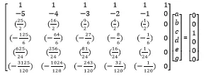
For find these coefficients, I used Matlab command window by storing values of A & B to get variable X values. The format I used is

X = inv(A)*B

Then, the output of the coefficients are

a = (-5/6)

b = 61/12

c = -13

d = (107/6)

e = (-77/6)

g = 15/4

Now, divide the hypothesis equation by Δx²

^{`(∂^2 u)/(∂x^2) = (a f(i-5) + b f(i-4) + c f(i-3) + d f(i-2) + e f(i-1) + g f(i))/(∆x^2)`}

Apply the coefficients to get the fourth order approximation

`(∂^2 u)/(∂x^2) = (((-5)/6) f(i-5) +(61/12) f(i-4) +(-13) f(i-3) +(107/6) f(i-2) +((-77)/6) f(i-1) +(15/4) f(i))/(∆x^2)`

From Taylor’s table, to know the unknown of the summation for the fifth & sixth order derivative write the equation by adding the values of the table of its own derivative as coefficient.

`(∂^2 u)/(∂x^2)` = (a + b + c + d + e + g) f(i) + (-5a – 4b -3c -2d -e) f’(i)Δx + ((e/2) + (4d/2) + (9c/2) + (16b/2) + (25a /2)) f’’(i) Δx² + ((-e/6) + (-8d/6) + (-27c/6) + (-64b/6) + (-125a /6)) f’’’(i) Δx³ + ((e/24) + (16d/24) + (81c/24) + (256b/24) + (625a/24)) f’’’(i) Δx⁴ + ((-e/120) + (-32d/120) + (-243c/120) + (-1024b/120) + (-3125a/120))f’’’’’(i) Δx⁵ + ((64d/720) + (e/720) + (729c/720) + (5096b/720) + (15625a/720))f’’’’’’(i) Δx⁶

Now, order of all is 0 except second derivative. In order to check it in in fifth & sixth, divide the above equation by Δx². Then, fifth one is become third derivative. So, the order of Δ³ is 0 as per known. It will get neglect. The sixth order become Δ⁴. Here, Δ⁴ is the truncation error for the fourth order. The final equation is

`(∂^2 u)/(∂x^2)` = ((e/2) + (4d/2) + (9c/2) + (16b/2) + (25a /2)) f’’(i) + ((64d/720) + (e/720) + (729c/720) + (5096b/720) + (15625a/720))f’’’’’’(i) Δx⁴

Code:

clear all
close all
clc

% given
x = pi/3;

% numerical derivative
dx = linspace(pi/4,pi/40000,20);

for i = 1:length(dx)

    central_difference_error(i) = central_difference(x,dx(i));
    skew_right_hand_side_error(i) = skew_right_hand_side_difference(x,dx(i));
    skew_left_hand_side_error(i) = skew_left_hand_side_difference(x,dx(i));

end

% plotting

figure (1)
loglog(dx,central_difference_error,'color','r')
hold on
loglog(dx,skew_right_hand_side_error,'color','b')
loglog(dx,skew_left_hand_side_error,'color','g')
legend('central difference error','skew right hand side error','skew left hand side error')
xlabel('dx')
ylabel('Truncation error')
title('4th order approximation of a 2nd order derivative')

function central_difference_error = central_difference(x,dx)

% analytical derivative 
% given analytical function = exp(x)*cos(x);
second_order_derivative = -2*exp(x)*sin(x);

% coefficients

a = - 1/12;
b = 4/3;
c = - 5/2;
d = 4/3;
e = - 1/12;

% fourth order approximation
central_difference = ((a*exp(x-2*dx)*cos(x-2*dx)) + (b*exp(x-dx)*cos(x-dx)) + (c*exp(x)*cos(x)) + (d*exp(x+dx)*cos(x+dx)) + (e*exp(x+2*dx)*cos(x+2*dx)))/(dx^2);

% truncation error
central_difference_error = abs(central_difference - second_order_derivative);

end

function skew_right_hand_side_error = skew_right_hand_side_difference(x,dx)

% analytical derivative 
% given analytical function = exp(x)*cos(x);
second_order_derivative = -2*exp(x)*sin(x);

% coefficients
a = 15/4;
b = (-77/6);
c = (107/6);
d = -13;
e = 61/12;
g = (-5/6);


% second order approximation
skew_right_hand_side_difference = ((a*exp(x)*cos(x)) + (b*exp(x+dx)*cos(x+dx)) + (c*exp(x+2*dx)*cos(x+2*dx)) + (d*exp(x+3*dx)*cos(x+3*dx)) + (e*exp(x+4*dx)*cos(x+4*dx) + (g*exp(x+5*dx)*cos(x+5*dx))))/(dx^2);

% truncation error
skew_right_hand_side_error = abs(skew_right_hand_side_difference - second_order_derivative);

end

function skew_left_hand_side_error = skew_left_hand_side_difference(x,dx)

% analytical derivative 
% given analytical function = exp(x)*cos(x);
second_order_derivative = -2*exp(x)*sin(x);

% coefficients
a = (-5/6);
b = 61/12;
c = -13;
d = (107/6);
e = (-77/6);
g = 15/4;


% fourth order approximation
skew_left_hand_side_difference = ((a*exp(x-5*dx)*cos(x-5*dx)) + (b*exp(x-4*dx)*cos(x-4*dx)) + (c*exp(x-3*dx)*cos(x-3*dx)) + (d*exp(x-2*dx)*cos(x-2*dx)) + (e*exp(x-dx)*cos(x-dx) + (g*exp(x)*cos(x))))/(dx^2);

% truncation error
skew_left_hand_side_error = abs(skew_left_hand_side_difference - second_order_derivative);

end

Explanation:

1. Initially, I provided the given input to solve this problem.
2. Create the new script to write a function for finding 4^th order of error for the different schemes.
3. Function file name must be in the name of the function and program file & function file must be in the same folder. If not, program shows error. One another method is that you can write the function at the end of the program too. It will be work perfectly.
4. Within the function script, equations to find the solution for the analytical derivate, 4^th order of approximation & truncation error must provide. Otherwise, it shows the error.
5. To get the solution for the order of error for the range of dx, created loop condition for the length of dx.
6. Within the loop, program will run till the length of dx & gets stop. The results will get stored in the workspace for the length of the dx.
7. Finally, for graphical representation I used “loglog” plotting command to show the least value comparision of error with respect to dx.

Skewed scheme is better because we cannot use the central scheme for one sided problems or not equal nodal points on each side from its centre node problems.

Result: