Week 3 - External flow simulation over an Ahmed body.

Objective:

The aim is to simulate the flow externally over the Ahmed body to determine the aerodynamic forces.

Ahmed body and it’s importance:

The Ahmed Body was first created by S.R. Ahmed in his research “Some Salient Features of the Time-Averaged Ground Vehicle Wake” in 1984. Since then, it has become a benchmark for aerodynamic simulation tools. The simple geometrical shape has a length of 1.044 meters, height of 0.288 meters, and a width of 0.389 meters. It also has 0.5-meter cylindrical legs attached to the bottom of the body and the rear surface has a slant that falls off at 40 degrees.

Fuel consumption of the car should be low and that’s how the product should be is expect by everybody from the car manufacturer. So, in order to satisfy this condition, the aerodynamic drag plays a vital role. Complexly shaped cars are very challenging to model and it’s difficult to quantify the aerodynamic drag computationally. The Ahmed body is a benchmark model widely used in the automotive industry for validating simulation tools. The Ahmed body shape is simple enough to model, while maintaining car-like geometry features.

Why the drag coefficient is important?

Because it quantifies the resistance of an object in a fluid environment. It is not an absolute constant for a body’s shape because it varies with the speed and direction of flow, object shape and size, and the density and viscosity of the fluid. The lower the drag coefficient of an object, the less aerodynamic or hydrodynamic drag occurs. In terms of a car, the lower the drag coefficient, the more efficient the car is. As well as affecting the top speed of a vehicle, the drag coefficient also affects the handling. Cars with a low drag coefficient are sought after, but decreasing the drag drastically can reduce the downforce and lead to loss in road traction and a higher chance of car accidents.

Most cars have an average drag coefficient of between 0.30 and 0.35.

Negative pressure in the wake region:

The flow behind an object separates from the surface and creates a highly turbulent region behind the object, called the wake. The pressure inside the wake region remains low as the flow separates and a net pressure force (pressure drag) is produced. In other words, due to the production of pressure drag being produced from flow separation, the pressure in the wake region is low. This is what is causing the vacuum.

Significance of a point of separation:

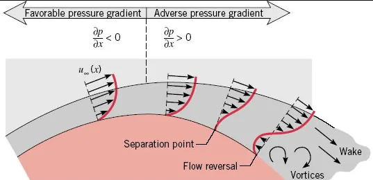
Flow separation is caused due to positive pressure gradient. The separation of the boundary layer takes place at the point where the wall shear stress becomes zero which is the starting point of the circulation.

When a fluid flows around a body, forces act between the fluid and the surface due to the viscosity. These intermolecular forces are the cause for the drag, among other things. However, due to the forces acting, the surface of the solid body also tries to bind the fluid to itself. This also leads to the fluid adhering to the surface (no-slip condition). The layer above this adherent fluid layer will not be able to simply tear itself away from it, because intermolecular attraction and pressure forces also act between the layers. As a result, any flow flowing around a body is tempted to follow the profile of the surface. As long as the contour of a body has smooth transitions and the internal cohesion of the fluid is large enough to resist the inertial forces, a flow can follow the contour.

In the case of sharp transitions or when flowing around blunt bodies, however, the fluid is often no longer able to follow the profile. The boundary layer or flow begins to detach itself from the body surface. This is referred to as a boundary layer separation or flow separation. Downstream of the separation point, vortices often form, resulting in a turbulent flow.

In order to reduce the drag force when fluid flows over the body, we need to have the smooth surface.

Case 1: Baseline mesh

Geometry:

Import the Ahmed body to space claim.

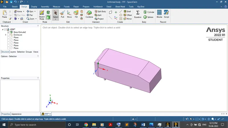
Go to prepare to create the enclosure around the Ahmed body.

Create the plane section at the origin. As the body is perfectly symmetric, we can run the simulation by considering the only half body. This is the best practice where you can save on the number of cells and get the results faster as well.

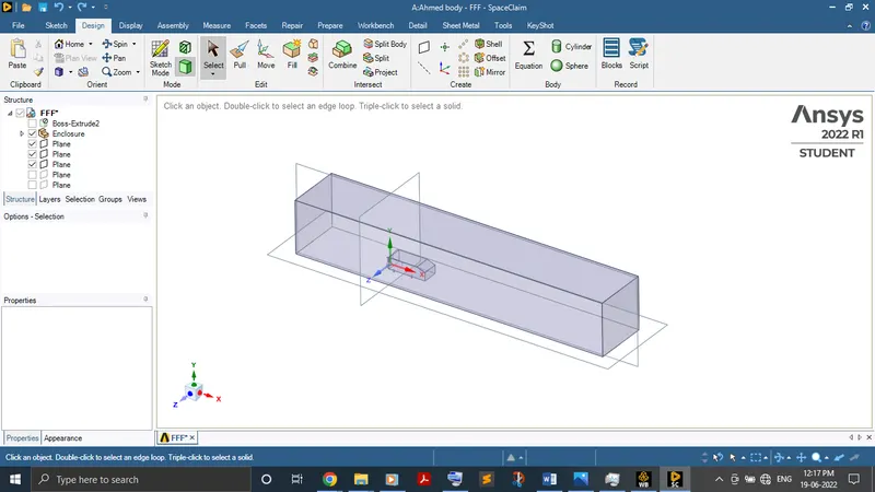
To split the body symmetrically, go to the design in space claim and use split body option.

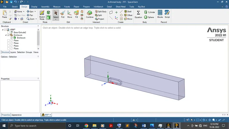
Finally, apply suppressed for physics to Ahmed body for not to affect the meshing result. If we don’t do it, the mesh will seem like a discontinuous and improper.

Meshing:

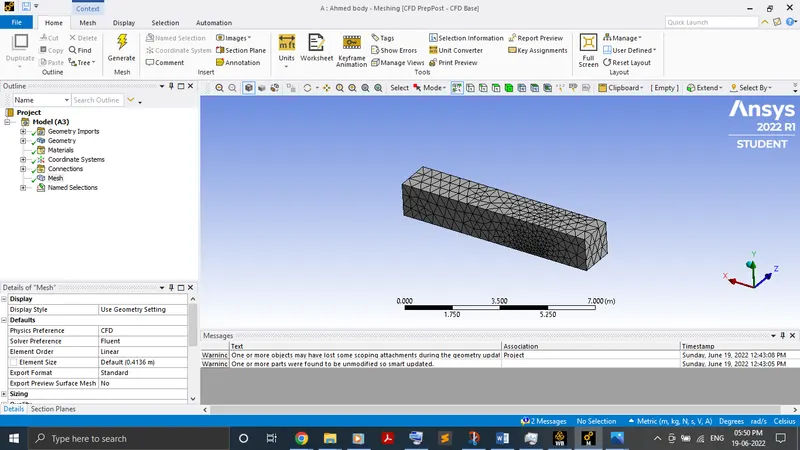
Select the faces of the enclosure and create boundary conditions by using named selection.

To create the boundary condition for the body, hide the enclosure faces by selecting it using F8. Select the body to name it by using box select.

Perform the simulation just with default mesh setting.

Setup:

Choose solver type as density based steady state.

Choose viscous model as K-epsilon turbulence model.

Continue with the default fluid material air.

Boundary conditions are

Velocity inlet – 25 (in m/s)

Pressure outlet – 0 (gauge pressure)

Wall – No slip condition

Reference values:

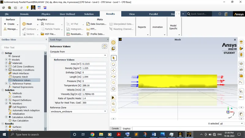
Create cut plane normal to z axis to witness the contour result on the plane.

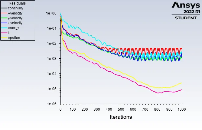
Intialize solution with hybrid initialization and run calculation till solution gets converge.

Result:

Residual plot:

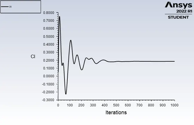
Lift co-efficient:

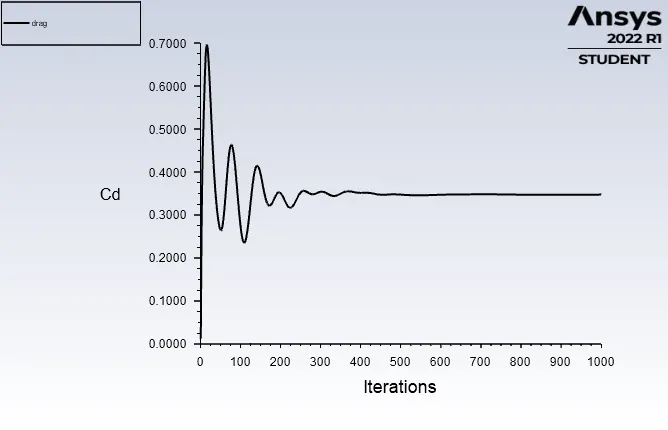
Drag co-efficient:

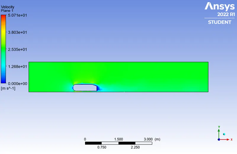
Velocity contour:

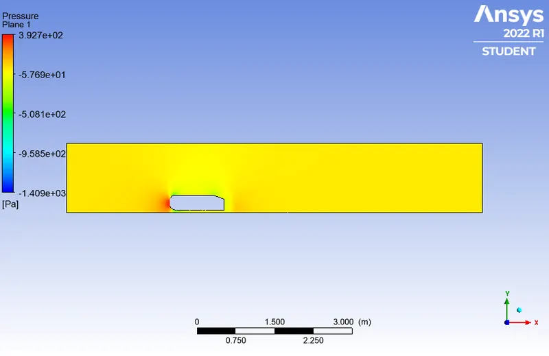
Pressure contour:

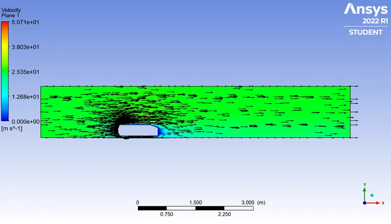
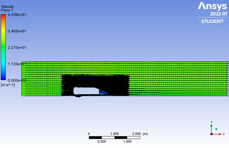
Velocity vector plot:

Case 2: Refining mesh

Case (a):

Geometry:

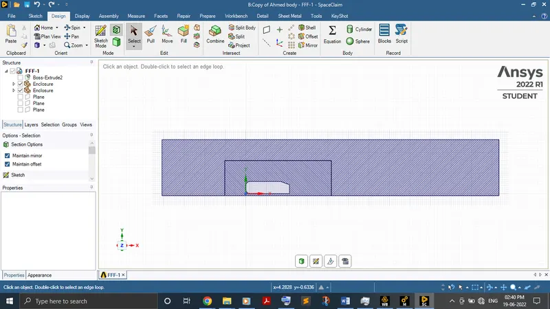
Add local refinement enclosure around the body. Then set the share topology to share for the purpose of sharing the information between the enclosures and also to make mesh result better.

Meshing:

Set the hexahedral mesh type by choosing multi zone method for the outer enclosure which helps to get high accuracy result.

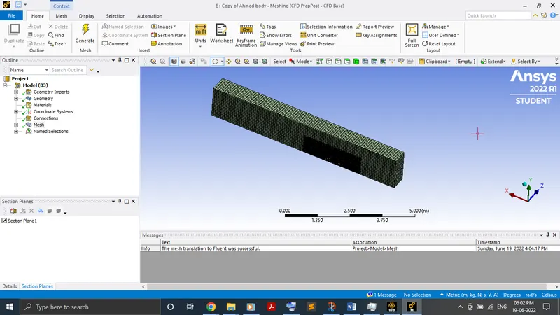
Element size (1^st enclosure) – 0.1 m

Maximum size (1^st enclosure) – 0.1 m

Next, set the body size by selecting the 2^nd enclosure and set the element size as 0.05 m.

Finally, set the face size for Ahmed body’s leg in the element size as 0.005 m.

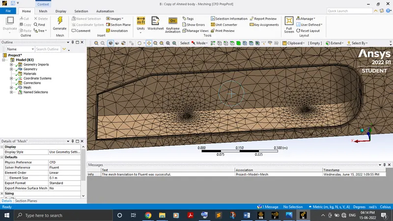
To capture the better result around the wall, create inflation by choosing total thickness as 15e-3 m to maximum of 1.2 m gap towards the end layer. Here, created the maximum layer of 5.

Setup:

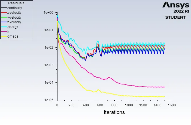
Here, setup is same as of case 1 except the viscous model. Here, simulation was done for the K-omega SST turbulence model.

Result:

Residual plot:

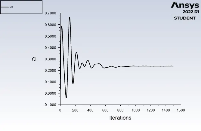
Lift co-efficient:

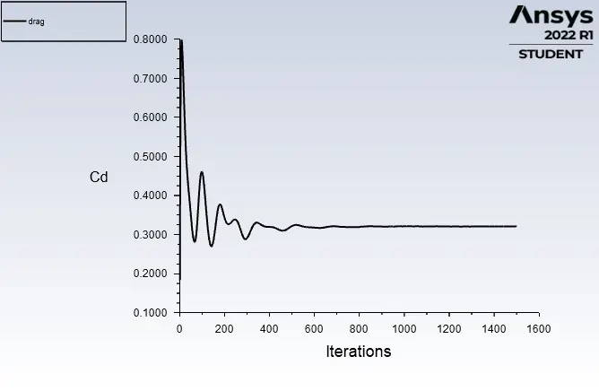
Drag co-efficient:

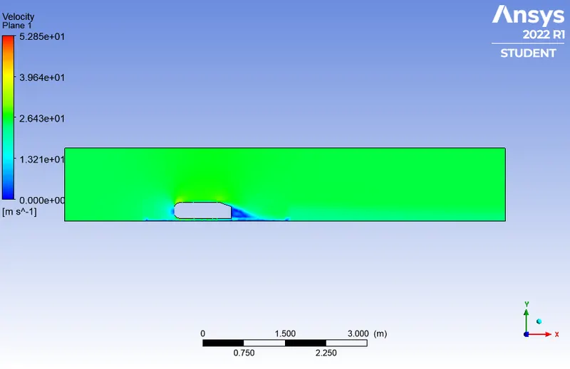
Velocity contour:

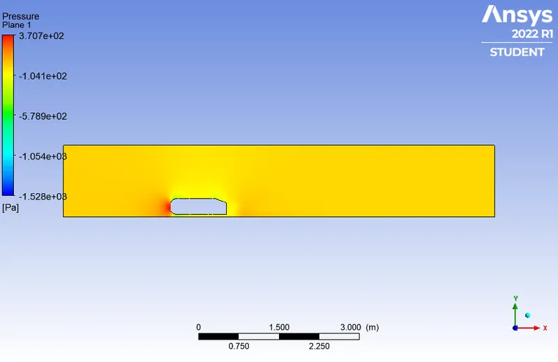
Pressure contour:

Velocity vector plot:

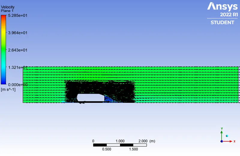
Case (b):

Everything is similar as of previous case, even to next case except meshing portion.

Meshing:

Element size (1^st enclosure) – 0.09 m

Maximum size (1^st enclosure) – 0.09 m

Element size (2^nd enclosure) – 0.045 m

Ahmed body’s leg face size – 0.005 m

To capture the better result around the wall, create inflation by choosing 1^st layer thickness inflation option and under that fix first layer height as 3e-3 m to maximum of 1.2 m gap towards the end layer. Here, created the maximum layer of 10.

Result:

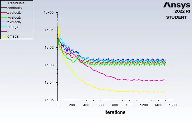
Residual plot:

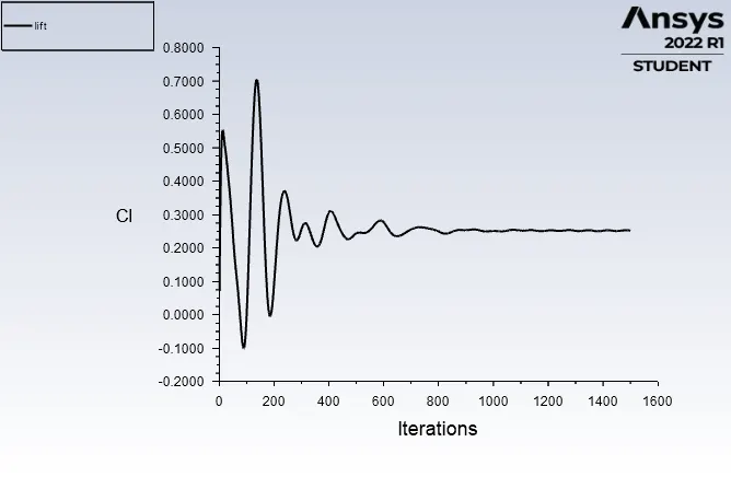
Lift co-efficient:

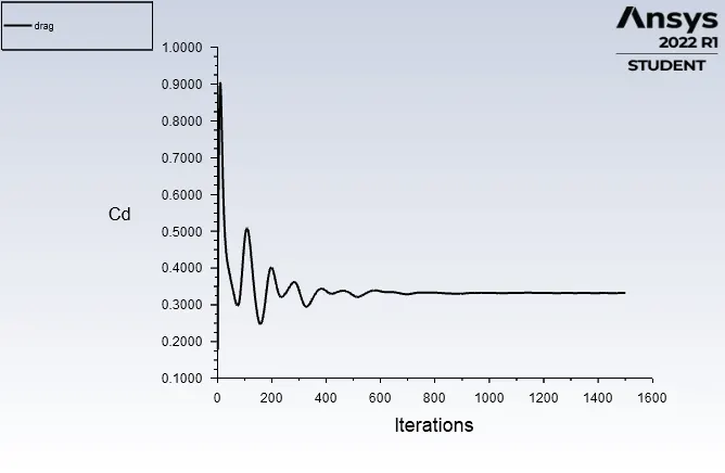
Drag co-efficient:

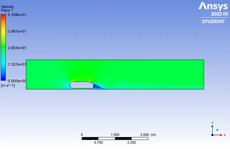
Velocity contour:

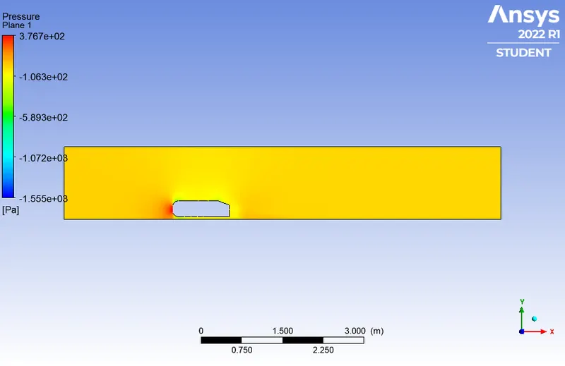
Pressure contour:

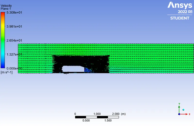
Velocity vector plot:

Case (c):

Meshing:

Element size (1^st enclosure) – 0.08 m

Maximum size (1^st enclosure) – 0.08 m

Element size (2^nd enclosure) – 0.04 m

Ahmed body’s leg face size – 0.005 m

To capture the better result around the wall, create inflation by choosing 1^st layer thickness inflation option and under that fix first layer height as 0.15e-3 m to maximum of 1.2 m gap towards the end layer. Here, created the maximum layer of 10.

Result:

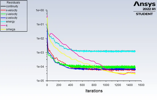
Residual plot:

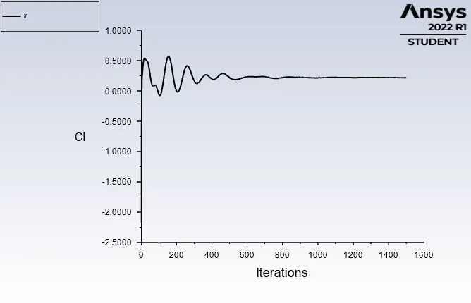
Lift co-efficient:

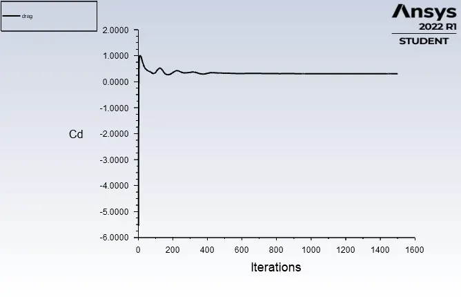
Drag co-efficient:

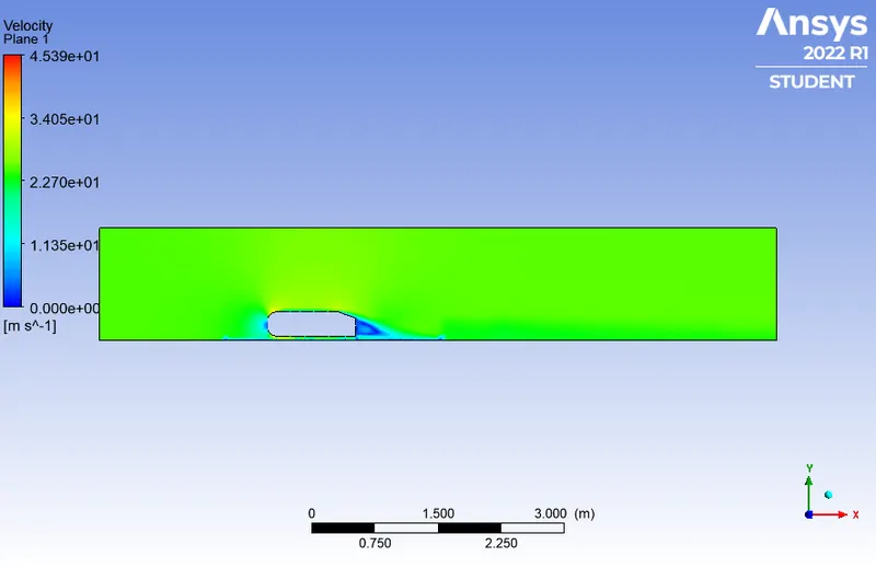
Velocity contour:

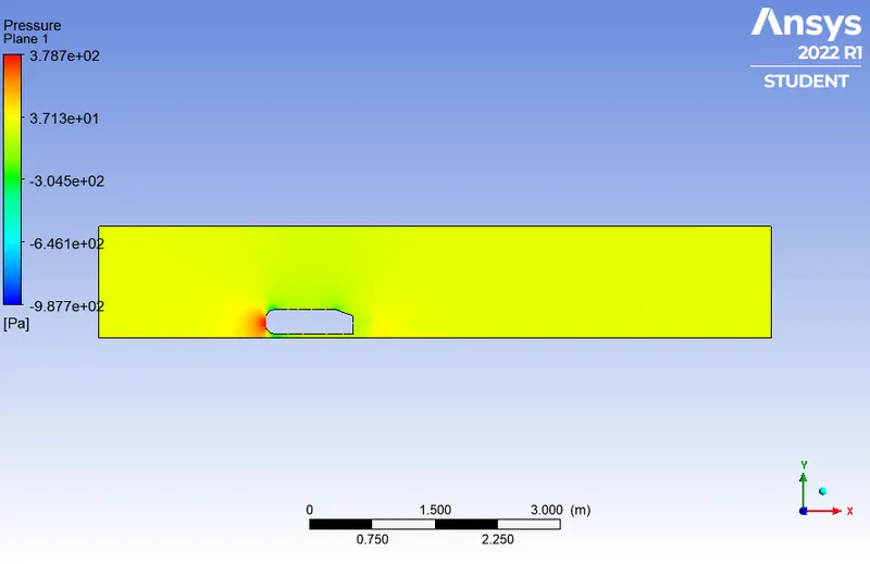
Pressure contour:

Velocity vector plot:

Grid independent test:

Comparison:

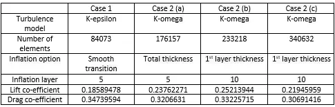
When the velocity is 25 m/s, the drag co-efficient should be around 0.33 which was obtained in case 2 (b). More the element size is small, the result will be accurate.

The difference between the K-epsilon and K-omega is that K-epsilon suits better to analyse the result of the flow which is away from the wall and K-omega suits better to analyse the result of the flow which takes place nearby the wall.

Conclusion:

• Grid independence test helps to find at what cell size the solution gets converged.
• Inflation option, inflation layer and turbulence model plays a vital role to solution gets converge.
• When mesh gets refined, drag and lift co-efficient starts to decrease.
• Beyond the point of separation, usually the flow gets separate. But here, the flow recirculate and attach to the boundary layer due to turbulence.
• Result satisfies the adverse pressure gradient.