Week 5.2 - Literature review: ODE Stability

Stability:

In mathematics, when the condition slightly gets a disturbance in the system doesn’t produce too disrupting effect on that system. In terms of the solution of a differential equation, a function f(x) is said to be stable if any other solution of the equation that starts out sufficiently close to it when x=0 remains close to it for succeeding values of x. If the difference between the solutions approaches zero as x increases, the solution is stable. If not, then it is called unstable.

In order to find the solution, we are using Euler method.

Euler method:

In mathematics and computational science, the Euler method is a first-order numerical procedure for solving differential equations with a given initial value. The most basic is explicit method for numerical integration of differential equations. The Euler method is a first-order method, which means that the local error (error per step) is proportional to the square of the step size, and the global error (error at a given time) is proportional to the step size. The Euler method often serves as the basis to construct more complex methods.

Methods to obtain stability:

Explicit & implicit are the methods used in numerical analysis for obtaining numerical approximation to the solution of time dependent differential equations.

Explicit method:

It calculate the state of a system at a later time from the state of the system at the current time.

Mathematically, consider ODE dy = dt*f(t,y)

Apply forward difference approach

y_n+1 - y_n = dt*f(t_n,y_n)

y_n+1 = y_n + dt*f(t_n,y_n)

Here, y_n is the current system state

y_n+1 is the later system state

dt is the small time step

We can program to find it by controlling either value of small time step or length of the small time step

1. When the small time step (dt) is large, error increases. Also has high chance of the system become unstable. If small time step is less, then the system is stable.
2. More the length of the small time step has stable system. If, it’s less then become unstable.

Implicit method:

It calculates both the state of a system at a later time as well as at the current time.

Mathematically, consider ODE dy = dt*f(x,t)

Apply backward difference approach

y_n - y_n-1 = dt*f(t_n,y_n)

y_n = y_n-1 + dt*f(t_n,y_n)

Here, y_n is the current system state

y_n-1 is the later system state

dt is the small time step

In this method, though value of small time step or length of the small time step, the solution is always stable. Simply, it’s stable in all the conditions.

Program by controlling length of the time step:

1. Explicit method:

# Explicit euler

import math
import matplotlib.pyplot as plt
import numpy as np

def f(t,y):
	return -1000*y - math.exp(-t)

t_start = 0
t_end = 0.1
n = 500
dt = (t_end - t_start)/(n-1)
print(dt)
t = 0
y_old = 0
y_new = []

for i in range (0,n):
	y_new.append(y_old + (dt*f(t, y_old)))
	y_old = y_new[i]
	t = t + dt

plt.plot(y_new)
plt.title('Length of the time step = 500')
plt.show()

Result:

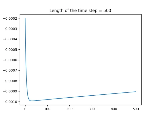
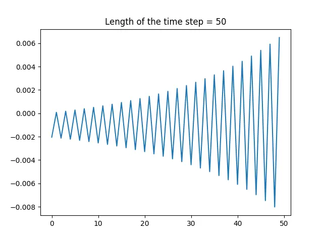
From the result obtained, we can see that when length of the time step is small the system become unstable. So, it must be large to maintain system as stable.

2. Implicit method:

# Implicit euler

import math
import matplotlib.pyplot as plt
import numpy as np

def f(t,y,dt):
	return (y - math.exp(-t)*dt)/(1+1000*dt)

t_start = 0
t_end = 0.1
n = 50
dt = (t_end - t_start)/(n-1)
print(dt)
t = 0
y_old = 0
y_new = []

for i in range (0,n):
	y_new.append((f(t, y_old, dt)))
	y_old = y_new[i]
	t = t + dt

plt.plot(y_new)
plt.title('Length of the time step = 50')
plt.show()

Result:

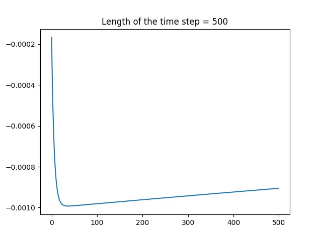
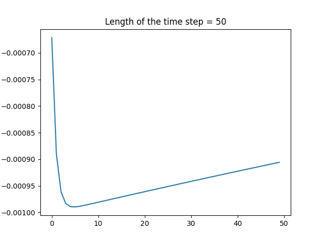
From the result obtained, the system is stable though condition changes.

Program by controlling time step:

import math
import matplotlib.pyplot as plt
import numpy as np

def explicit_euler(total_t,dt):
	t = np.arange(0,total_t,dt)
	y = np.zeros(len(t))

	for i in range (1,len(t)):
		y[i] = y[i-1] + dt*(-1000*y[i-1] - np.exp(-t[i-1]))

	return [t,y]


def implicit_euler(total_t,dt):
	t = np.arange(0,total_t,dt)
	y = np.zeros(len(t))

	for i in range (1,len(t)):
		y[i] = (y[i-1] - np.exp(-t[i-1])*dt)/(1+1000*dt)

	return [t,y]

total_t = 0.1
dt = 1.9e-4
t,y_explicit = explicit_euler(total_t,dt)
t,y_implicit = implicit_euler(total_t,dt)
plt.plot(t,y_explicit)
plt.plot(t,y_implicit)
plt.title('When time step is small(dt = 1.9e-4)')
plt.legend(['Explicit','Implicit'])
plt.show()

Result:

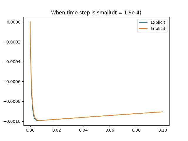
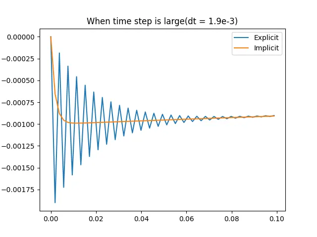
From the result obtained, the stability is maintain in implicit method but when small time step become large the solution become unstable in explicit method.

Answers to the questions by relate it from the obtained results of program:

1. ODE become unstable only in the explicit condition when programmed code by controlling small time step or length of the small time step. When small time steps has large value, the system become unstable. Also system become unstable, when the value of length of the small time step is less.
2. When the stability criteria doesn’t satisfied before the start of the engineering simulation, the result will blow away. Though the criteria gets satisfied, the result we are going to obtain by simulation is always approximate only. Also, possibility of minimal error in the result.
3. Of course, stability condition can be derived for all types of problems. But here, we are using difference schemes like forward, backward, central to obtain the result.