Week 7 - Simulation of a 1D Super-sonic nozzle flow simulation using Macormack Method
Objective: The aim is to simulate the isentropic flow through a quasi 1D subsonic-supersonic nozzle and converge the solution for both conservative & non-conservative forms of governing equation using MacCromack’s technique.
Theory: Generally, Nozzle & pipe is working based on the principle of Bernoulli’s theorem. Here, when the gas flow reaches the inlet of the nozzle from reservoir, it starts to flow within nozzle as a subsonic flow (M<1) in the convergent portion. When the flow reaches the throat, then it will become sonic (M=1). Generally, the area of the convergent portion is decreasing. So, velocity starts to increase and pressure decrease at every time step. But, as per Bernoulli’s theorem when the area increases velocity decreases. It suits for the pipe flow. When it comes to CD nozzle, in the divergence portion when area increases velocity also increases but pressure keep decreases. This is because of expansion. So, at the exit the flow is supersonic (M>1).
MacCromack’s method: It is an explicit finite difference method which is second order accurate and widely used discretization scheme for numerical solution.
It has two types of steps to solve the solution. They are
- Predictor step
- Corrector step
Predictor step: Here, we use the forward difference scheme to obtain the new solution by replacing old solution for the variables at different time step and space step.
Corrector step: Here, we use the backward difference scheme to obtain the solution by replacing old solution for the variables at different time step and space step.
Conservative form:
Governing equations:
Continuity equation:
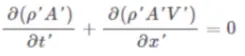
Momentum equation:

Energy equation:

Initial conditions:
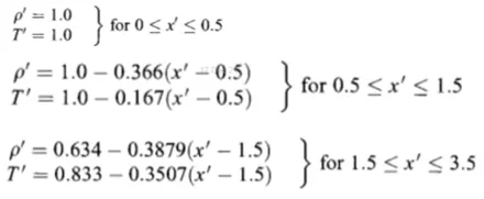
Store the governing equations of all as a transformed manner into the solution variable “U” & flux term “F”.
Create the time loop within the function and initialize the flux term. Then, start the predictor step within the space loop for all the governing equation and update the solution.
Primitive variables:
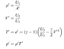
At the outside space loop, calculate the primitive solution and update the flux term.
Then, start the corrector step again within the space loop for all the governing equation.
Compute the average time derivate between predictor & corrector.
Again, at the outside space loop, initialize the boundary condition for inlet & outlet.
Finally, update the primitive solution & final solution. Plot the results for length of the nozzle(x) & primitive variables.
Non-conservative form:
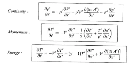
Governing equations:
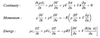
Transform the equations into non-dimensionalized equations
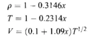
Initial conditions:
Repeat the steps of conservative form and converge the solution.
Code:
clear all
close all
clc

% Inputs
n = 31;
x = linspace(0,3,n);
dx = x(2) - x(1);
gamma = 1.4;

% Throat node
throat_node = ((n-1)/2)+1;

% Area
A = 1+(2.2*(x-1.5).^2);

% Time steps
nt = 1000;

[non_con,rho,V,T,M_nc,machnumber_nc,P_nc,rho_throat_node_nc,V_throat_node_nc,T_throat_node_nc,P_throat_node_nc,M_throat_node_nc,machnumber_throat_node_nc] = non_conv(x,A,gamma,dx,nt,n,throat_node);

figure(3)
subplot(5,1,1)
plot(x,machnumber_nc,'b')
ylabel('Mach number')
title('Variables difference along X for non conservative form')
subplot(5,1,2)
plot(x,P_nc,'b')
ylabel('P')
subplot(5,1,3)
plot(x,rho,'b')
ylabel('Density')
subplot(5,1,4)
plot(x,V,'b')
ylabel('V')
subplot(5,1,5)
plot(x,T,'b')
xlabel('X')
ylabel('Temperature')

[con,rho,V,T,M_c,machnumber_c,P_c,rho_throat_node_c,V_throat_node_c,T_throat_node_c,P_throat_node_c,M_throat_node_c,machnumber_throat_node_c] = conv(x,gamma,dx,nt,n,throat_node);

figure(4)
subplot(5,1,1)
plot(x,machnumber_c,'b')
ylabel('Mach number')
title('Variables difference along X for conservative form')
subplot(5,1,2)
plot(x,P_c,'b')
ylabel('P')
subplot(5,1,3)
plot(x,rho,'b')
ylabel('Density')
subplot(5,1,4)
plot(x,V,'b')
ylabel('V')
subplot(5,1,5)
plot(x,T,'b')
xlabel('X')
ylabel('Temperature')

figure(5)
subplot(5,1,1)
plot(machnumber_throat_node_nc,'b')
hold on
plot(machnumber_throat_node_c,'r')
ylabel('Mach number')
title('Variables difference at throat for various time steps')
legend('Non conservative','Conservative')
subplot(5,1,2)
plot(P_throat_node_nc,'b')
hold on
plot(P_throat_node_c,'r')
ylabel('P')
subplot(5,1,3)
plot(rho_throat_node_nc,'b')
hold on
plot(rho_throat_node_c,'r')
ylabel('Density')
subplot(5,1,4)
plot(V_throat_node_nc,'b')
hold on
plot(V_throat_node_c,'r')
ylabel('V')
subplot(5,1,5)
plot(T_throat_node_nc,'b')
hold on
plot(T_throat_node_c,'r')
xlabel('X')
ylabel('Temperature')

figure(6)
plot(x,M_nc,"Color",'b')
hold on
plot(x,M_c,"Color",'r')
xlabel('X')
ylabel('Mass flow rate')
legend('Non conservative','Conservative')
title('Comparison of mass flow rate')

function [non_con,rho,V,T,M_nc,machnumber_nc,P_nc,rho_throat_node_nc,V_throat_node_nc,T_throat_node_nc,P_throat_node_nc,M_throat_node_nc,machnumber_throat_node_nc] = non_conv(x,A,gamma,dx,nt,n,throat_node)

% Calculate initial profile
rho = 1 - (0.3146*x);
T = 1 - (0.2314*x);
V = (0.1+(1.09.*x)).*(T.^(0.5));
CFL = 0.5;
dt = min(CFL.*((dx)./((T.^0.5)+V)));

tic
% Outer time loop
for k = 1:nt

    rho_old = rho;
    V_old = V;
    T_old = T;

    % Predictor method

    for j = 2:(n-1)

        dV_dx = (V(j+1)-V(j))/dx;
        drho_dx = (rho(j+1)-rho(j))/dx;
        dT_dx = (T(j+1)-T(j))/dx;
        dlogA_dx = (log(A(j+1))-log(A(j)))/dx;

        % Continuity equation
        drho_dt_p(j) = (-rho(j)*dV_dx) - (rho(j)*V(j)*(dlogA_dx)) - (V(j)*(drho_dx));

        % Momentum equation
        dV_dt_p(j) = (-V(j)*(dV_dx)) - ((1/gamma)*((dT_dx) + ((T(j)/rho(j))*(drho_dx))));

        % Energy equation
        dT_dt_p(j) = (-V(j)*(dT_dx)) - ((gamma-1)*T(j)*((dV_dx)+(V(j)*(dlogA_dx))));

        % Solution update
        rho(j) = rho(j) + (drho_dt_p(j)*dt);
        V(j) = V(j) + (dV_dt_p(j)*dt);
        T(j) = T(j) + (dT_dt_p(j)*dt);
    end

    % Corrector method

    for j = 2:(n-1)

        dV_dx = (V(j)-V(j-1))/dx;
        drho_dx = (rho(j)-rho(j-1))/dx;
        dT_dx = (T(j)-T(j-1))/dx;
        dlogA_dx = (log(A(j))-log(A(j-1)))/dx;

        % Continuity equation
        drho_dt_c(j) = (-rho(j)*dV_dx) - (rho(j)*V(j)*(dlogA_dx)) - (V(j)*(drho_dx));

        % Momentum equation
        dV_dt_c(j) = (-V(j)*(dV_dx)) - ((1/gamma)*((dT_dx) + ((T(j)/rho(j))*(drho_dx))));

        % Energy equation
        dT_dt_c(j) = (-V(j)*(dT_dx)) - ((gamma-1)*T(j)*((dV_dx)+(V(j)*(dlogA_dx))));

    end

    % Compute the average time derivative

    drho_dt = 0.5*(drho_dt_p + drho_dt_c);
    dV_dt = 0.5*(dV_dt_p + dV_dt_c);
    dT_dt = 0.5*(dT_dt_p + dT_dt_c);

    % Final solution update
    for i = 2:(n-1)
        rho(i) = rho_old(i) + (drho_dt(i)*dt);
        V(i) = V_old(i) + (dV_dt(i)*dt);
        T(i) = T_old(i) + (dT_dt(i)*dt);
    end

    % Apply the boundary condition
    % Inlet
    V(1) = (2*V(2)) - V(3);

    % Outlet
    rho(n) = (2*rho(n-1)) - rho(n-2);
    V(n) = (2*V(n-1)) - V(n-2);
    T(n) = (2*T(n-1)) - T(n-2);

    % Calculate mass flow, mach number & pressure
    M_nc = rho.*A.*V;
    P_nc = rho.*T;
    machnumber_nc = V./(T.^0.5);

    rho_throat_node_nc(k) = rho(throat_node);
    V_throat_node_nc(k) = V(throat_node);
    T_throat_node_nc(k) = T(throat_node);
    M_throat_node_nc(k) = M_nc(throat_node);
    P_throat_node_nc(k) = P_nc(throat_node);
    machnumber_throat_node_nc(k) = machnumber_nc(throat_node);

    figure(1)
    if k==250
        plot(x,M_nc,"Color",'b')
        hold on
    elseif k==500
        plot(x,M_nc,'Color','g')
        hold on
    elseif k==1000
        plot(x,M_nc,'Color','r')
        hold on
        xlabel('X')
        ylabel('Massflow')
        title('Mass flow through the nozzle at various time steps - Non conservative form')
        legend('250','500','1000')
    end

end

non_con = toc;

end

function [con,rho,V,T,M_c,machnumber_c,P_c,rho_throat_node_c,V_throat_node_c,T_throat_node_c,P_throat_node_c,M_throat_node_c,machnumber_throat_node_c] = conv(x,gamma,dx,nt,n,throat_node)

% Calculate initial profile
% x between 0 - 0.5
for i = 1:n
    if (x(i) >=0 && x(i)<=0.5)
        rho(i) = 1;
        T(i) = 1;
    end
end

% x between 0.5 - 1.5
for i = 1:n
    if (x(i) >=0.5 && x(i)<=1.5)
        rho(i) = 1 - (0.366*(x(i)-0.5));
        T(i) = 1 - (0.167*(x(i)-0.5));
    end
end

% x between 1.5 - 3.5
for i = 1:n
    if (x(i) >=1.5 && x(i)<=3.5)
        rho(i) = 0.634 - (0.3879*(x(i)-1.5));
        T(i) = 0.833 - (0.3507*(x(i)-1.5));
    end
end

A = 1 + (2.2*(x-1.5).^2);
V = (0.59)./(rho.*A);

% Calculate initial condition
U1 = (rho.*A);
U2 = (rho.*A.*V);
U3 = U1.*(((T)./(gamma-1))+((0.5*gamma)*(V.^2)));

CFL = 0.5;
dt = min(CFL.*((dx)./((T.^0.5)+V)));

tic
% Outer time loop
for k = 1:nt

    U1_old = U1;
    U2_old = U2;
    U3_old = U3;

    % Initializing Flux
    F1 = U2;
    F2 = (U2.^2./U1) + (((gamma-1)./gamma)*(U3-((0.5*gamma)*((U2.^2)./U1))));
    F3 = ((gamma.*U2.*U3)./U1) - ((0.5*gamma*(gamma-1)*(U2.^3))./(U1.^2));

    % Predictor method
    for j = 2:(n-1)

        dF1_dx(j) = (F1(j+1) - F1(j))/dx;
        dF2_dx(j) = (F2(j+1) - F2(j))/dx;
        dF3_dx(j) = (F3(j+1) - F3(j))/dx;
        J2(j) = (1/gamma)*rho(j)*T(j)*((A(j+1)-A(j))/dx);

        % Continuity equation
        dU1_dt_p(j) = -(dF1_dx(j));

        % Momentum equation
        dU2_dt_p(j) = -(dF2_dx(j))+J2(j);

        % Energy equation
        dU3_dt_p(j) = -(dF3_dx(j));

        % Solution update
        U1(j) = U1(j) + (dU1_dt_p(j)*dt);
        U2(j) = U2(j) + (dU2_dt_p(j)*dt);
        U3(j) = U3(j) + (dU3_dt_p(j)*dt);

    end

    % Primitives
    rho = (U1./A);
    V = (U2./U1);
    T = (gamma-1).*((U3./U1)-((0.5.*gamma).*(V.^2)));

    % Flux update
    F1 = U2;
    F2 = (U2.^2./U1) + (((gamma-1)./gamma)*(U3-((gamma/2)*((U2.^2)./U1))));
    F3 = ((gamma.*U2.*U3)./U1) - (gamma*(gamma-1)*(U2.^3))./(2*(U1.^2));

    % Corrector method
    for l = 2:(n-1)

        dF1_dx(l) = (F1(l) - F1(l-1))/dx;
        dF2_dx(l) = (F2(l) - F2(l-1))/dx;
        dF3_dx(l) = (F3(l) - F3(l-1))/dx;
        J2(l) = (1/gamma)*rho(l)*T(l)*((A(l)-A(l-1))/dx);

        % Continuity equation
        dU1_dt_c(l) = -(dF1_dx(l));

        % Momentum equation
        dU2_dt_c(l) = -(dF2_dx(l))+J2(l);

        % Energy equation
        dU3_dt_c(l) = -(dF3_dx(l));

    end

    % Compute the average time derivative
    dU1_dt = 0.5*(dU1_dt_p+dU1_dt_c);
    dU2_dt = 0.5*(dU2_dt_p+dU2_dt_c);
    dU3_dt = 0.5*(dU3_dt_p+dU3_dt_c);

    % Inlet boundary condition
    U1(1) = (rho(1)*A(1));
    U2(1) = (2*U2(2))-U2(3);
    U3(1) = U1(1)*(((T(1))/(gamma-1))+((0.5*gamma)*(V(1)^2)));

    % Outlet boundary condition
    U1(n) = (2*(U1(n-1)))-U1(n-2);
    U2(n) = (2*(U2(n-1)))-U2(n-2);
    U3(n) = (2*(U3(n-1)))-U3(n-2);

    % Final update
    for m = 2:(n-1)
        U1(m) = U1_old(m) + (dU1_dt(m)*dt);
        U2(m) = U2_old(m) + (dU2_dt(m)*dt);
        U3(m) = U3_old(m) + (dU3_dt(m)*dt);
    end

    % Primitives
    rho = (U1./A);
    V = (U2./U1);
    T = (gamma-1).*((U3./U1)-((0.5.*gamma).*(V.^2)));

    % Calculate mass flow, mach number & pressure
    M_c = rho.*A.*V;
    P_c = rho.*T;
    machnumber_c = V./(T.^0.5);

    rho_throat_node_c(k) = rho(throat_node);
    V_throat_node_c(k) = V(throat_node);
    T_throat_node_c(k) = T(throat_node);
    M_throat_node_c(k) = M_c(throat_node);
    P_throat_node_c(k) = P_c(throat_node);
    machnumber_throat_node_c(k) = machnumber_c(throat_node);

    figure(2)
    if k==250
        plot(x,M_c,"Color",'b')
        hold on
    elseif k==500
        plot(x,M_c,'Color','g')
        hold on
    elseif k==1000
        plot(x,M_c,'Color','r')
        hold on
        xlabel('X')
        ylabel('Massflow')
        title('Mass flow through the nozzle at various time steps - Conservative form')
        legend('250','500','1000')
    end

end

con = toc;

end
Grid independence test:
Value of end time step at throat:
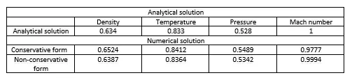
Non-conservative form is more accurate than the conservative form due to residual.
1. Steady-state distribution of primitive variables inside the nozzle:Result:
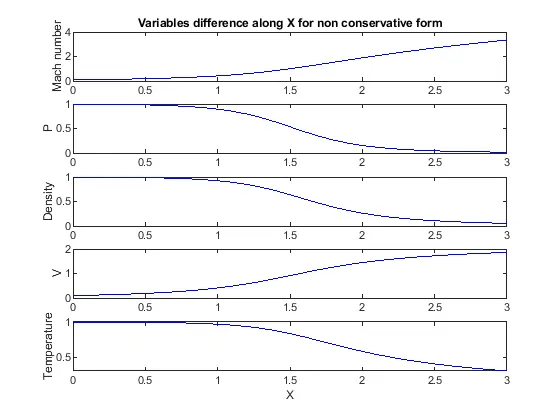
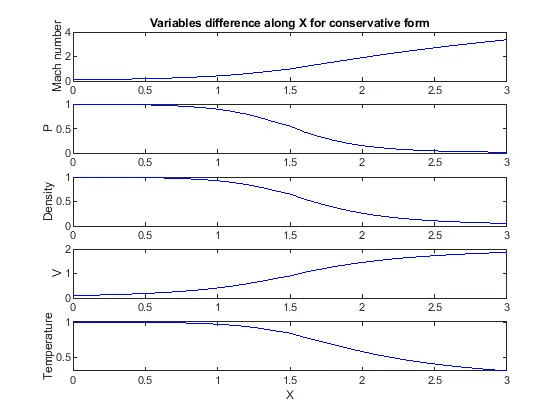
This result satisfies the bernoulli's theorem.
2. Time-wise variation of the primitive variables
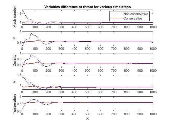
Conservative form converge the solution quicker than the non conservative form. Variation of the variables changes less for the conservative form than non conservative form.
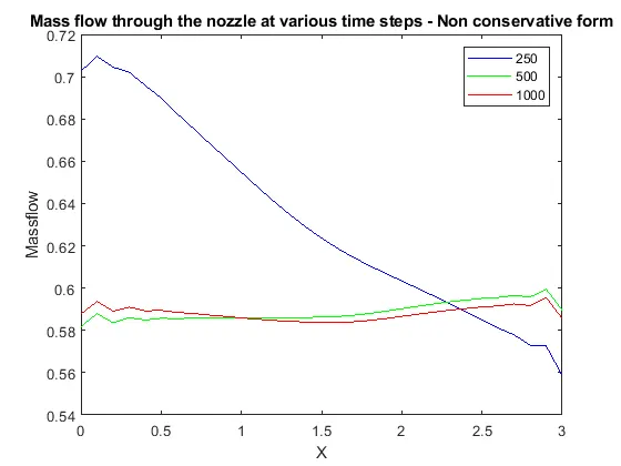
3. Variation of Mass flow rate distribution inside the nozzle at different time steps during the time-marching process
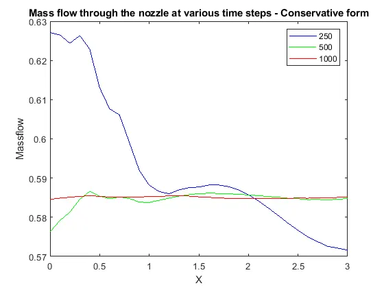
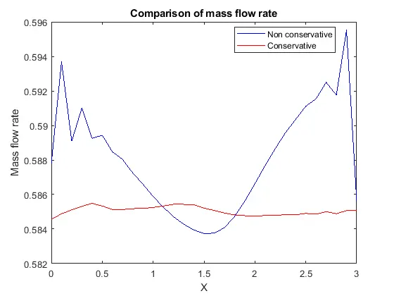
4. Comparison of Normalized mass flow rate distributions of both forms