Week 11 - Simulation of Flow through a pipe in OpenFoam
Hydrodynamic entrance:
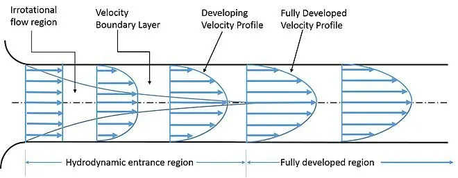
The hydrodynamic entrance region refers to the area of a pipe where fluid entering a pipe develops a velocity profile due to viscous forces propagating from the interior wall of a pipe. This region is characterized by a non-uniform flow. The fluid enters a pipe at a uniform velocity, then fluid particles in the layer in contact with the surface of the pipe come to a complete stop due to the no-slip condition. Due to viscous forces within the fluid, the layer in contact with the pipe surface resists the motion of adjacent layers and slows adjacent layers of fluid down gradually, forming a velocity profile. For the conservation of mass to hold true, the velocity of layers of the fluid in the centre of the pipe increases to compensate for the reduced velocities of the layers of fluid near the pipe surface. This develops a velocity gradient across the cross-section of the pipe. When the fluid just enters the pipe, the thickness of the boundary layer gradually increases from zero moving in the direction of fluid flow and eventually reaches the pipe centre and fills the entire pipe. This region from the entrance of the pipe to the point where the boundary layer covers the entire pipe is termed as the hydrodynamic entrance region and the length of the pipe in this region is termed as the hydrodynamic entry length. In this region, the velocity profile develops and thus the flow is called the hydrodynamically developing flow. After this region, the velocity profile is fully developed and continues unchanged. This region is called the hydrodynamically fully developed region. But this is not the fully developed fluid flow until the normalized temperature profile also becomes constant.
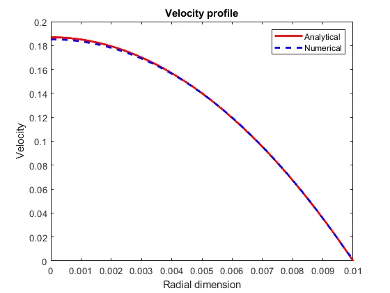
Here our case is incompressible laminar flow, the velocity profile in the fully developed region is parabolic but in the case of turbulent flow it gets a little flatter due to vigorous mixing in radial direction and eddy motion. The velocity profile remains unchanged in the fully developed region.
The hydrodynamic entry length for the laminar flow is to be calculated by the following formula
entry_L = 0.0575*Re*D
Hagen–Poiseuille equation:
The Hagen–Poiseuille equation is a physical law that gives the pressure drop in an incompressible and Newtonian fluid in laminar flow flowing through a long cylindrical pipe of constant cross section
The assumptions of the equation are that the fluid is incompressible and Newtonian; the flow is laminar through a pipe of constant circular cross-section that is substantially longer than its diameter; and there is no acceleration of fluid in the pipe. For velocities and pipe diameters above a threshold, actual fluid flow is not laminar but turbulent, leading to larger pressure drops than calculated by the Hagen–Poiseuille equation.
The pressure drop can be calculated by using the following formula which is from the Hagen-Poiseuille equation
Δp = (8*µ*L*Vavg)/R2
The average velocity can be calculated from the Reynold’s number
Vavg = (Re*nu)/D
where, nu = µ/ρ which is Kinematic viscosity
µ - Dynamic viscosity
ρ – Density
The maximum velocity can be calculated by the following formula
Vmax = 2*Vavg
Shear stress:
Shear stress is primarily caused by friction between fluid particles, due to fluid viscosity. Fluids at rest cannot resist a shear stress; in other words, when a shear stress is applied to a fluid at rest, the fluid will not remain at rest, but will move because of the shear stress.
τ = µ*(du/dx)
MatLab Code to create blockMeshDict:
clear all
close all
clc

% assumptions
Re = 2100;                     % Reynold's number
rho = 1000;                    % Density of water
D = 0.02;                      % assumed diameter
R = 0.01;                      % Radius
mu = 0.00089;                  % Dynamic viscosity of water
nu = mu/rho;                   % Kinematic viscosity
entry_L = 0.0575*Re*D;         % Hydrodynamic entrance length
L = entry_L + 0.3;             % Total length of the pipe
theta = 3;                     % Wedge angle

% boundary conditions
v_avg = (Re*nu)/D;             % average velocity
v_max = 2*v_avg;               % maximum velocity

% vertices
v0 = [0 0 0];
v1 = [0 (R*cosd(0.5*theta)) (-R*sind(0.5*theta))];
v2 = [0 (R*cosd(0.5*theta)) (R*sind(0.5*theta))];
v3 = [L 0 0];
v4 = [L (R*cosd(0.5*theta)) (-R*sind(0.5*theta))];
v5 = [L (R*cosd(0.5*theta)) (R*sind(0.5*theta))];

% blockMeshDict file creation
f1 = fopen('blockMeshDict.txt','w');

% headlines
fprintf(f1,'/*--------------------------------*- C++ -*----------------------------------* \n');
fprintf(f1,'   =========             	  |\n');
fprintf(f1,'   \\  	   /  F ield     	  | OpenFOAM: The Open Source CFD Toolbox \n');
fprintf(f1,'    \\	  /   O peration 	  | Website:  https://openfoam.org \n');
fprintf(f1,'     \\   /	  A nd       	  | Version:  9 \n');
fprintf(f1,'      \\ / 	  M anipulation   | \n');
fprintf(f1,'*---------------------------------------------------------------------------*/ \n');
fprintf(f1,'FoamFile \n');
fprintf(f1,'{ \n');
fprintf(f1,'	format  	ascii; \n');
fprintf(f1,'	class   	dictionary; \n');
fprintf(f1,'	object  	blockMeshDict; \n');
fprintf(f1,'} \n');
fprintf(f1,'// * * * * * * * * * * * * * * * * * * * * * * * * * * * * * * * * * * * * * // \n');
fprintf(f1,'\n');

% convert to meters
fprintf(f1,'convertToMeters 1; \n');
fprintf(f1,'\n');

% vertices
fprintf(f1,'vertices \n');
fprintf(f1,'( \n');
fprintf(f1,'        (%f %f %f) \n', v0);
fprintf(f1,'        (%f %f %f) \n', v1);
fprintf(f1,'        (%f %f %f) \n', v2);
fprintf(f1,'        (%f %f %f) \n', v3);
fprintf(f1,'        (%f %f %f) \n', v4);
fprintf(f1,'        (%f %f %f) \n', v5);
fprintf(f1,'); \n');
fprintf(f1,'\n');

% blocks
fprintf(f1,'blocks \n');
fprintf(f1,'( \n');
fprintf(f1,'	hex (0 1 2 0 3 4 5 3) (50 1 200) simpleGrading (1 1 1) \n');
fprintf(f1,'); \n');
fprintf(f1,'\n');

% edges
fprintf(f1,'edges \n');
fprintf(f1,'( \n');
fprintf(f1,'	arc 1 2 (%f %f %f) \n',v0(1),R,v0(3));
fprintf(f1,'	arc 4 5 (%f %f %f) \n',v3(1),R,v3(3));
fprintf(f1,'); \n');
fprintf(f1,'\n');

% boundary
fprintf(f1,'boundary \n');
fprintf(f1,'( \n');
fprintf(f1,'	inlet \n');
fprintf(f1,'	{ \n');
fprintf(f1,'    	type patch; \n');
fprintf(f1,'    	faces \n');
fprintf(f1,'    	( \n');
fprintf(f1,'    	     (0 1 2 0) \n');
fprintf(f1,'    	); \n');
fprintf(f1,'	} \n');
fprintf(f1,'	outlet \n');
fprintf(f1,'	{ \n');
fprintf(f1,'    	type patch; \n');
fprintf(f1,'    	faces \n');
fprintf(f1,'    	( \n');
fprintf(f1,'    	     (3 4 5 3) \n');
fprintf(f1,'    	); \n');
fprintf(f1,'	} \n');
fprintf(f1,'	front \n');
fprintf(f1,'	{ \n');
fprintf(f1,'    	type wedge; \n');
fprintf(f1,'    	faces \n');
fprintf(f1,'    	( \n');
fprintf(f1,'    	     (0 3 4 1) \n');
fprintf(f1,'    	); \n');
fprintf(f1,'	} \n');
fprintf(f1,'	back \n');
fprintf(f1,'	{ \n');
fprintf(f1,'    	type wedge; \n');
fprintf(f1,'    	faces \n');
fprintf(f1,'    	( \n');
fprintf(f1,'    	     (3 0 2 5) \n');
fprintf(f1,'    	); \n');
fprintf(f1,'	} \n');
fprintf(f1,'	pipe \n');
fprintf(f1,'	{ \n');
fprintf(f1,'    	type wall; \n');
fprintf(f1,'    	faces \n');
fprintf(f1,'    	( \n');
fprintf(f1,'    	     (1 4 5 2) \n');
fprintf(f1,'    	); \n');
fprintf(f1,'	} \n');
fprintf(f1,'	axis \n');
fprintf(f1,'	{ \n');
fprintf(f1,'    	type empty; \n');
fprintf(f1,'    	faces \n');
fprintf(f1,'    	( \n');
fprintf(f1,'    	     (0 3 3 0) \n');
fprintf(f1,'    	); \n');
fprintf(f1,'	} \n');
fprintf(f1,'); \n');
fprintf(f1,'\n');

% mergepatchpairs
fprintf(f1,'mergePatchPairs \n');
fprintf(f1,'( \n');
fprintf(f1,'); \n');
fprintf(f1,'\n');

fprintf(f1,'// ************************************************************************* // \n');

fclose(f1);
BlockMeshDict file:
/*--------------------------------*- C++ -*----------------------------------*
   =========             	  |
   \  	   /  F ield     	  | OpenFOAM: The Open Source CFD Toolbox
    \	  /   O peration 	  | Website:  https://openfoam.org
     \   /	  A nd       	  | Version:  9
      \ / 	  M anipulation   |
*---------------------------------------------------------------------------*/
FoamFile
{
	format  	ascii;
	class   	dictionary;
	object  	blockMeshDict;
}
// * * * * * * * * * * * * * * * * * * * * * * * * * * * * * * * * * * * * * //

convertToMeters 1;

vertices
(
        (0.000000 0.000000 0.000000)
        (0.000000 0.009997 -0.000262)
        (0.000000 0.009997 0.000262)
        (2.715000 0.000000 0.000000)
        (2.715000 0.009997 -0.000262)
        (2.715000 0.009997 0.000262)
);

blocks
(
	hex (0 1 2 0 3 4 5 3) (50 1 200) simpleGrading (1 1 1)
);

edges
(
	arc 1 2 (0.000000 0.010000 0.000000)
	arc 4 5 (2.715000 0.010000 0.000000)
);

boundary
(
	inlet
	{
    	type patch;
    	faces
    	(
    	     (0 1 2 0)
    	);
	}
	outlet
	{
    	type patch;
    	faces
    	(
    	     (3 4 5 3)
    	);
	}
	front
	{
    	type wedge;
    	faces
    	(
    	     (0 3 4 1)
    	);
	}
	back
	{
    	type wedge;
    	faces
    	(
    	     (3 0 2 5)
    	);
	}
	pipe
	{
    	type wall;
    	faces
    	(
    	     (1 4 5 2)
    	);
	}
	axis
	{
    	type empty;
    	faces
    	(
    	     (0 3 3 0)
    	);
	}
);

mergePatchPairs
(
);

// ************************************************************************* //
Steps for simulation:
- Initially, copy the cavity folder from the OpenFoam tutorials which is inside the incompressible folder, then in icoFoam folder by using the command “cp –r (folder name)/ $FOAM_RUN/(new folder name)” in the terminal window. To reach the tutorial folder from run folder just type the command “tut” in the terminal window. To see the list inside the folder type the command “ls”.
- Go to the run folder by typing “cd $FOAM_RUN” in the terminal window where we are going to run the simulation by copying the folder from the tutorials without change anything in it because that may lead to some collapse and we can’t recover it back. Only solution is re-installing OpenFoam.
- Inside the cavity folder, 0 folder has p & U text files. Constant folder has transport properties file. Finally, system folder has blockMeshDict, controlDict files. These are the required files to do the simulation by changing the things as per our problem required.
- To create the wedge geometry, open the blockMeshDict file with the help of the command “gedit” and arrange the vertices as per right hand thumb rule. Then, assign the type for the inlet & outlet as patches. For front and back, assign empty. For no slip walls(top), assign as wall. Finally, save the file.
- Open the pressure & velocity file, where assign the inlet conditions for the pressure is zero gradient & for the velocity is fixed value. At outlet, it’s vice versa. For front and back, both type are wedge. For no slip walls(top), pressure type is zero gradient and velocity type is no slip. Finally, axis type for both is empty & save the files.
- Open the transport properties file, where change the value of nu as 0.89e-6 to solve the solution for the laminar viscous flow which helps to obtain the courant number less than or equal to 0.5 till the simulation ends.
- Open the controlDict file to set the simulation timings, interval between each timings, time steps as per requirement.
- Command “./Allrun” in the terminal window to run the simulation. Now, go inside the folder & then type “paraFoam” to see the para view of the given geometry.
- Run the simulation in the para view.
- By using plot over line, measure the velocity profile for different cases.
- To get the shear stress in paraview, use calculator option and provide the name array. Then, in filters go to the search where type gradient unstructured data and type enter. In this provide the array name and gradient value of kinematic viscosity. Finally, create an another calculator to get the result.
Pressure file:
/*--------------------------------*- C++ -*----------------------------------*\
  =========                 |
  \\      /  F ield         | OpenFOAM: The Open Source CFD Toolbox
   \\    /   O peration     | Website:  https://openfoam.org
    \\  /    A nd           | Version:  9
     \\/     M anipulation  |
\*---------------------------------------------------------------------------*/
FoamFile
{
    format      ascii;
    class       volScalarField;
    object      p;
}
// * * * * * * * * * * * * * * * * * * * * * * * * * * * * * * * * * * * * * //

dimensions      [0 2 -2 0 0 0 0];

internalField   uniform 0;

boundaryField
{
    inlet
    {
        type            zeroGradient;
    }

    outlet
    {
        type            fixedValue;
        value           uniform 0;
    }

    front
    {
        type            wedge;
    }

    back
    {
        type            wedge;
    }

    top
    {
        type            zeroGradient;
    }

    axis
    {
        type            empty;
    }
}

// ************************************************************************* //
ControlDict file:
/*--------------------------------*- C++ -*----------------------------------*\
  =========                 |
  \\      /  F ield         | OpenFOAM: The Open Source CFD Toolbox
   \\    /   O peration     | Website:  https://openfoam.org
    \\  /    A nd           | Version:  9
     \\/     M anipulation  |
\*---------------------------------------------------------------------------*/
FoamFile
{
    format      ascii;
    class       dictionary;
    location    "system";
    object      controlDict;
}
// * * * * * * * * * * * * * * * * * * * * * * * * * * * * * * * * * * * * * //

application     icoFoam;

startFrom       startTime;

startTime       0;

stopAt          endTime;

endTime         25;

deltaT          0.01;

writeControl    timeStep;

writeInterval   20;

purgeWrite      0;

writeFormat     ascii;

writePrecision  6;

writeCompression off;

timeFormat      general;

timePrecision   6;

runTimeModifiable true;


// ************************************************************************* //
Transport properties file:
Here, provide the calculated kinematic viscosity value.
/*--------------------------------*- C++ -*----------------------------------*\
  =========                 |
  \\      /  F ield         | OpenFOAM: The Open Source CFD Toolbox
   \\    /   O peration     | Website:  https://openfoam.org
    \\  /    A nd           | Version:  9
     \\/     M anipulation  |
\*---------------------------------------------------------------------------*/
FoamFile
{
    format      ascii;
    class       dictionary;
    location    "constant";
    object      transportProperties;
}
// * * * * * * * * * * * * * * * * * * * * * * * * * * * * * * * * * * * * * //

nu              [0 2 -1 0 0 0 0] 0.89e-06;


// ************************************************************************* //
Velocity file:
Here, provide the calculated average velocity value at the inlet as fixed value.
/*--------------------------------*- C++ -*----------------------------------*\
  =========                 |
  \\      /  F ield         | OpenFOAM: The Open Source CFD Toolbox
   \\    /   O peration     | Website:  https://openfoam.org
    \\  /    A nd           | Version:  9
     \\/     M anipulation  |
\*---------------------------------------------------------------------------*/
FoamFile
{
    format      ascii;
    class       volVectorField;
    object      U;
}
// * * * * * * * * * * * * * * * * * * * * * * * * * * * * * * * * * * * * * //

dimensions      [0 1 -1 0 0 0 0];

internalField   uniform (0 0 0);

boundaryField
{
    inlet
    {
        type            fixedValue;
        value           uniform (0.09345 0 0);
    }

    outlet
    {
        type            zeroGradient;
    }

    front
    {
        type            wedge;
    }

    back
    {
        type            wedge;
    }

    top
    {
        type            noSlip;
    }

    axis
    {
        type            empty;
    }
}

// ************************************************************************* //
Paraview Results:
Variation of Velocity profile at various distances:
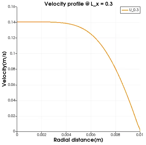
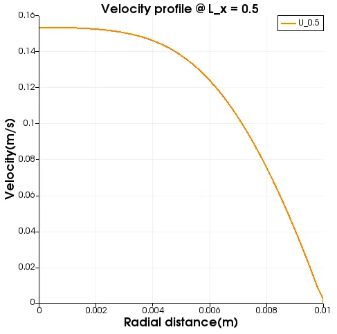
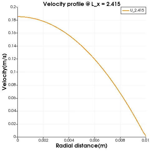
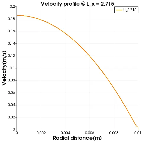
Initially, velocity in the entrance zone keep changes at minimal distance because of flow is not fully developed. Once, we achieved it the solution of the velocity will become converge.
Pressure at fully developed region:
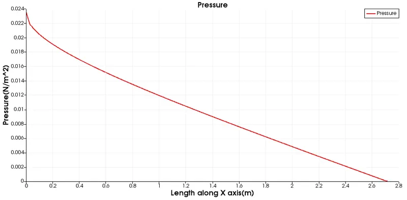
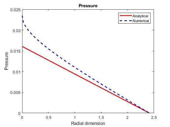
This satisfying the Bernoulli's theorem. So, result is perfect.
Shear stress:
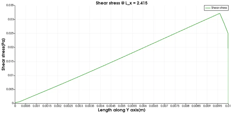
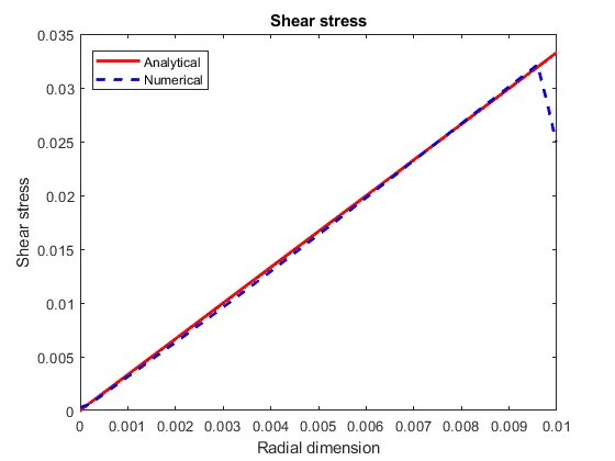
This shows that the shear nearby the wall is high than the other points. This is due to viscous.
MatLab code for analytical and numerical comparison:
clear all
close all
clc

% Inputs and analytical calculations
Re = 2100;                               % Reynold's number
rho = 1000;                              % Density of water
D = 0.02;                                % assumed diameter
R = 0.01;                                % Radius
mu = 0.00089;                            % Dynamic viscosity of water
nu = mu/rho;                             % Kinematic viscosity
entry_L = 0.0575*Re*D;                   % Hydrodynamic entrance length
L = entry_L + 0.3;                       % Total length of the pipe
L_r = linspace(0,R,1000);                % Radial distance
v_avg = (Re*nu)/D;                       % average velocity
v_max = 2*v_avg;                         % Maximum velocity
v_r = v_max*(1-((L_r.^2)/(R.^2)));       % Velocity gradient
L_p = linspace(0,entry_L,1000);          % entrance length
dp = (8*v_avg*mu*L_p)/(R^2);             % Pressure drop at the end of entrance length
kine_pressure = dp/rho;                  % Kinematic pressure
Tau = (2*mu*v_max*L_r)/(R^2);            % Shear stress
kine_pressure = fliplr(kine_pressure);

% Reading data file exported from paraview and numerical calculations
f1 = fopen('excel.csv','r');
B = fgetl(f1);
for i = 1:1000
    c = fgetl(f1);
    d = strsplit(c,',');
    vel(i) = d(1);
    pressure(i) = d(4);
    shear_stress(i) = d(12);
    length(i) = d(8);
    length_x(i) = d(7);
end

% To convert from cells
vel = str2double(vel);
pressure = str2double(pressure);
length = str2double(length);
length_x = str2double(length_x);
shear_stress = str2double(shear_stress);

% Plotting
figure(1)
plot(L_r,v_r,'r','LineWidth',2)
hold on
plot(length,vel,'color','b','LineWidth',2,'LineStyle','--')
title('Velocity profile')
xlabel('Radial dimension')
ylabel('Velocity')
legend('Analytical','Numerical')

figure(2)
plot(L_p,kine_pressure,'r','LineWidth',2)
hold on
plot(length_x,pressure,'color','b','LineWidth',2,'LineStyle','--')
title('Pressure')
xlabel('Radial dimension')
ylabel('Pressure')
legend('Analytical','Numerical')

figure(3)
plot(L_r,Tau,'r','LineWidth',2)
hold on
plot(length,shear_stress,'color','b','LineWidth',2,'LineStyle','--')
title('Shear stress')
xlabel('Radial dimension')
ylabel('Shear stress')
legend('Analytical','Numerical')
Result:
The results are approximately similar for both the methods