Week 8 - Simulating Cyclone separator with Discrete Phase Modelling

Aim: To perform analysis on cyclone separator and calculate the separation efficiency and pressure drop.

Cyclone separation:

Cyclone separation is a method of removing particulates from an air, gas or liquid stream, without the use of filters, through vortex separation. When removing particulate matter from liquid, a hydrocyclone is used; while from gas, a gas cyclone is used. Rotational effects and gravity are used to separate mixtures of solids and fluids. The method can also be used to separate fine droplets of liquid from a gaseous stream.

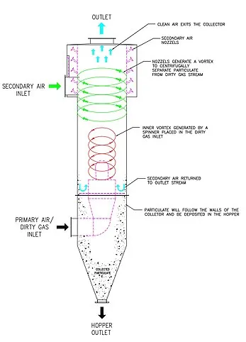
Four empirical models:

1. Iozia and Leith Model:

Iozia and Leith logistic model is a modified version of Barth Model, which is developed based on force balance. The model assumes that a particle carried by the vortex endures the influence of two forces: a centrifugal force, Z and a flow resistance, W. The collection efficiency ɳi of particle diameter dpi can be calculated from

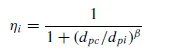
β is an expression for slope parameter derived based on the statistical analysis of experimental data of a cyclone with D = 0.25 m given as

and d_pc is the 50% cut size given by Barth

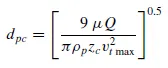
where core length, z_c, and core diameter, d_c, are given as

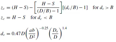
2. Li and Wang Model

The Li and Wang model includes particle bounce or re-entrainment and turbulent diffusion at the cyclone wall. A two-dimensional analytical expression of particle distribution in the cyclone is obtained. Li and Wang model was developed based on the following assumptions:

• The radial particle velocity and the radial concentration profile are not constant for uncollected particles within the cyclone.
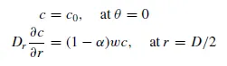
• Boundary conditions with the consideration of turbulent diffusion coefficient and particle bounce re-entrainment on the cyclone wall are:

• The tangential velocity is related to the radius of cyclone by: uRⁿ = constant.

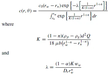
The concentration distribution in a cyclone is given as:

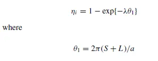
The resultant expression of the collection efficiency for particle of any size is given as

3. Koch and Licht Model

Koch and Licht collection theory recognized the inherently turbulent nature of cyclones and the distribution of gas residence times within the cyclone. Koch and Licht described particle motion in the entry and collection regions with the additional following assumptions:

• The tangential velocity of a particle is equal to the tangential velocity of the gas flow, i.e. there is no slip in the tangential direction between the particle and the gas.
• The tangential velocity is related to the radius of cyclone by: uRⁿ = constant.

A force balance and an equation on the particles collection yields the grade efficiency ɳ_i.

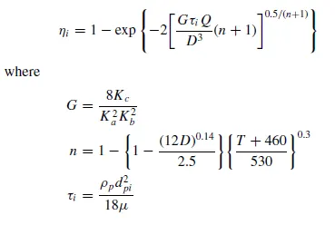
G is a factor related to the configuration of the cyclone, n is related to the vortex and τ is the relaxation term.

4. Lapple Model

Lapple model was developed based on force balance without considering the flow resistance. Lapple assumed that a particle entering the cyclone is evenly distributed across the inlet opening. The particle that travels from inlet half width to the wall in the cyclone is collected with 50% efficiency. The semi empirical relationship developed by Lapple to calculate a 50% cut diameter, dpc, is

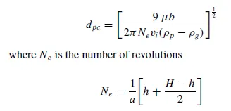
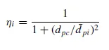
The efficiency of collection of any size of particle is given by

Solving & modelling approach:

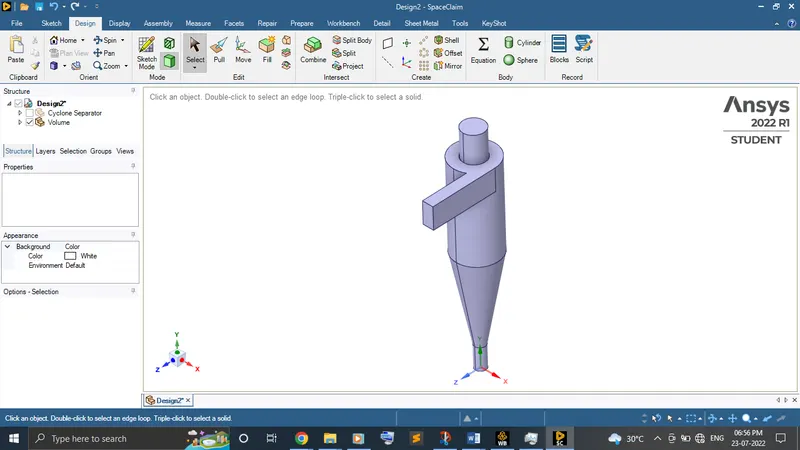
• Import the 3D cyclone separator geometry in space claim.
• Use volume extract option to extract the fluid volume.
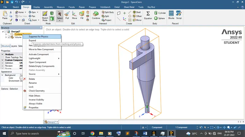
• Use suppress for physics on solid volume for not to take a part in meshing.
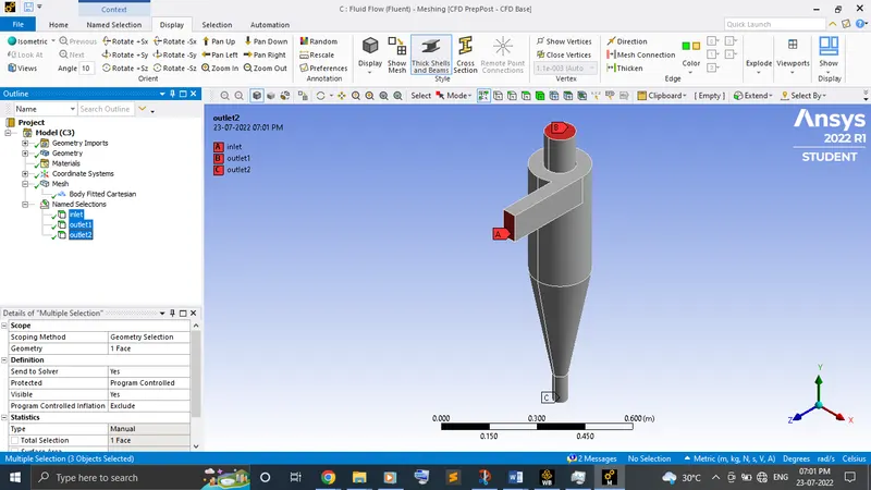
• Load the geometry in meshing. Do the named selections for the inlet and outlets. Mesh the geometry by inserting body method and choose Cartesian mesh.
• Do the necessary physics and boundary conditions setup in setup to converge the solution.
• Finally, compare the result of each case.

Pre-processing and solver setting:

Geometry:

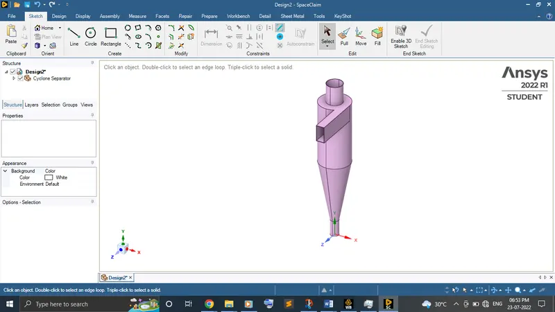
Import the 3D cyclone separator geometry in space claim.

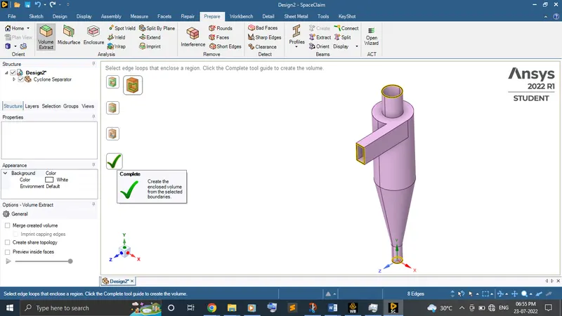
Use volume extract option by selecting the edges of the fluid zone to extract the fluid volume.

Use suppress for physics on solid volume for not to take a part in meshing.

Meshing:

Load the geometry in meshing and do the named selections for the faces.

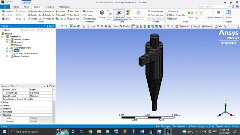
Do the mesh to the geometry for the following

Element size - 0.005 m

Mesh method – Cartesian

An attractive alternative to conventional body-fitted or unstructured meshing techniques is offered by the Cartesian cut cell approach. It allows for rapid, automatic, mesh generation for complex geometries, and maintains the computational conveniences offered by the use of Cartesian grids.

Nodes – 135094

Element - 122565

Setup:

Solver type - Steady state pressure based with gravity (y = -9.81 m/s²)

Model -

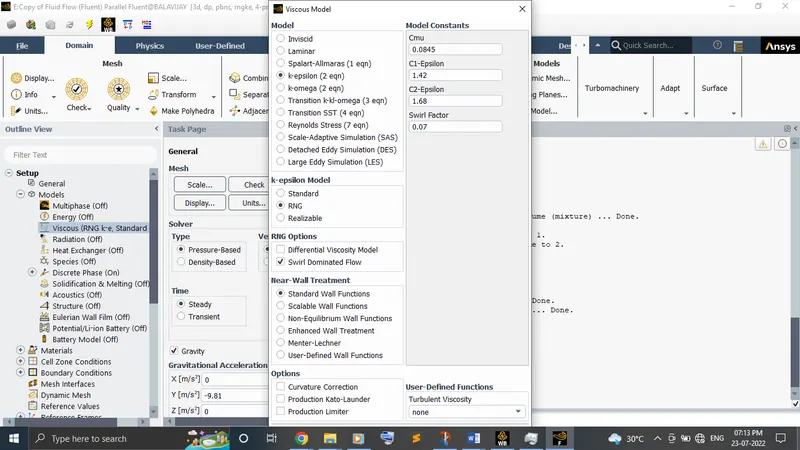
• RNG with swirl dominated flow, K-Epsilon viscous turbulence model with standard wall treatment.
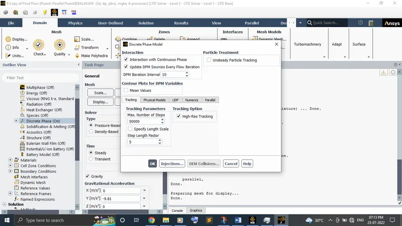
• DPM - interaction with continuous phase
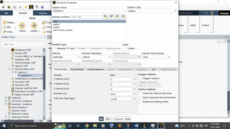
• Injections - Type (surface), Injection (inlet), Material (anthracite), Velocity (1 to 5 m/s), Diameter of the particle (1 to 5 micrometre)

Boundary Conditions - Inlet and wall (Reflect), Outlet 1 (Escape), Outlet 2 (Trap)

Initialize the standard initialization and run the calculation.

Separation efficiency:

The ratio of the number of the particles trapped to the number of the particles tracked.

Pressure drop:

It’s nothing but the difference between the two different points of pressure. Here, the difference between the inlet and the outlet 1 points of pressure.

Δp = Inlet - Outlet 1

Result:

1. Varying particle size with constant velocity:

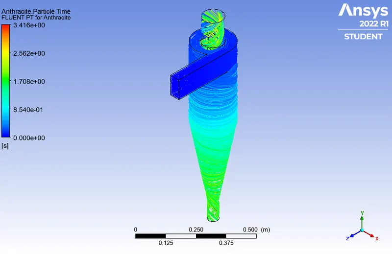
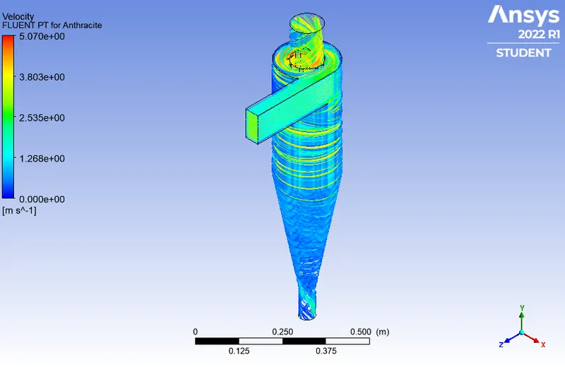
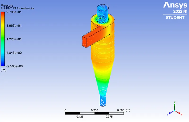
a. 1 µm:

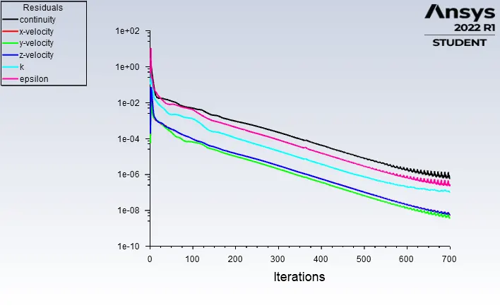
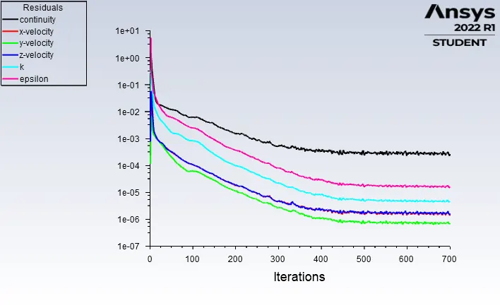
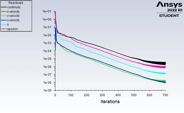
Residual plot:

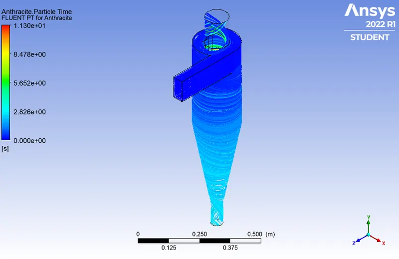
Anthracite particle contour:

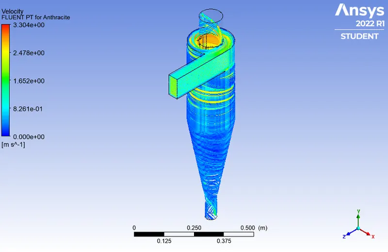
Velocity contour:

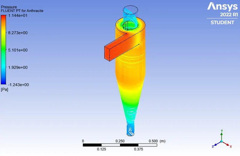
Pressure contour:

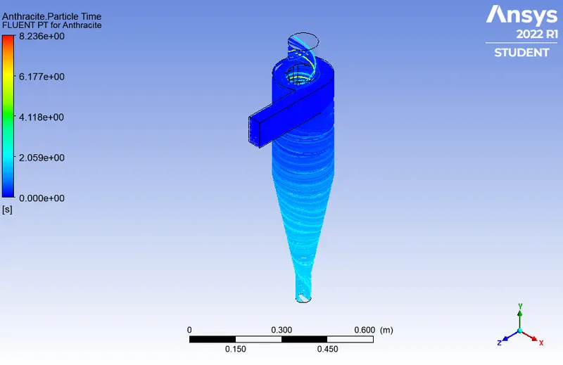
b. 2 µm:

Residual plot:

Anthracite particle contour:

Velocity contour:

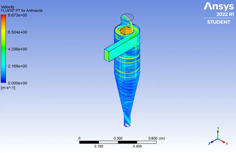
Pressure contour:

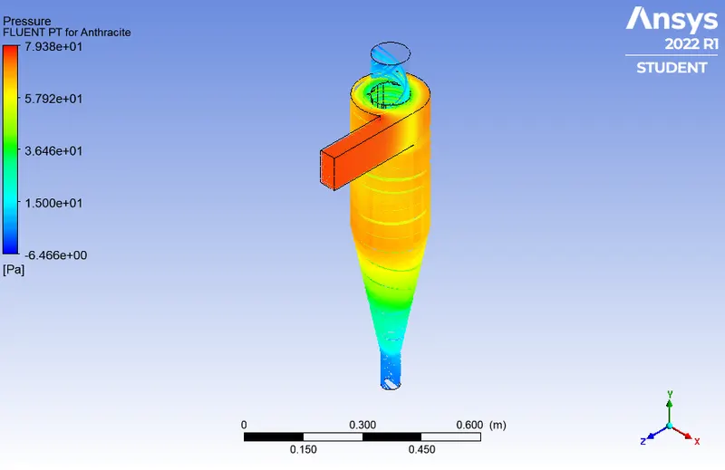
c. 3 µm:

Residual plot:

Anthracite particle contour:

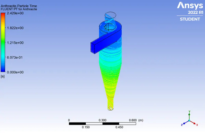
Velocity contour:

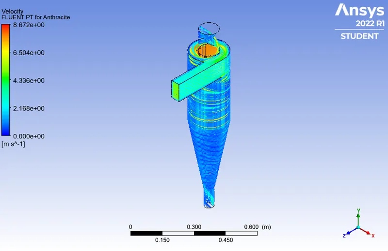
Pressure contour:

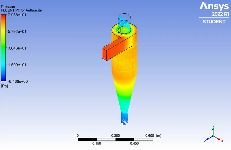
d. 4 µm:

Residual plot:

Anthracite particle contour:

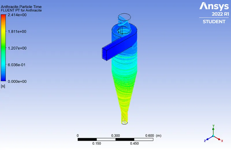
Velocity contour:

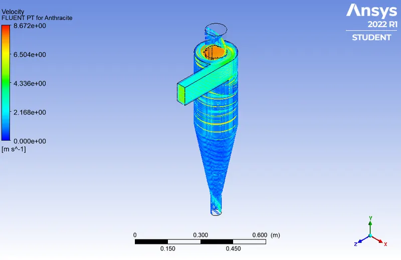
Pressure contour:

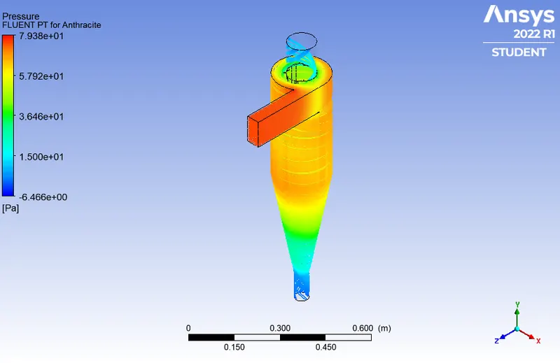
e. 5 µm:

Residual plot:

Anthracite particle contour:

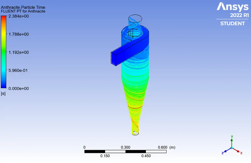
Velocity contour:

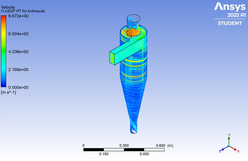
Pressure contour:

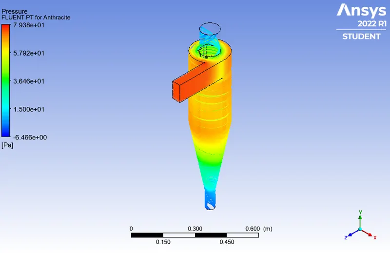
2. Varying velocity with constant particle size:

a. 1 m/s:

Residual plot:

Anthracite particle contour:

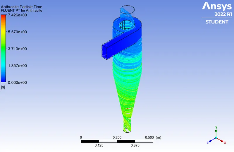
Velocity contour:

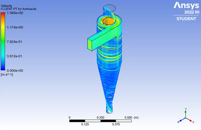
Pressure contour:

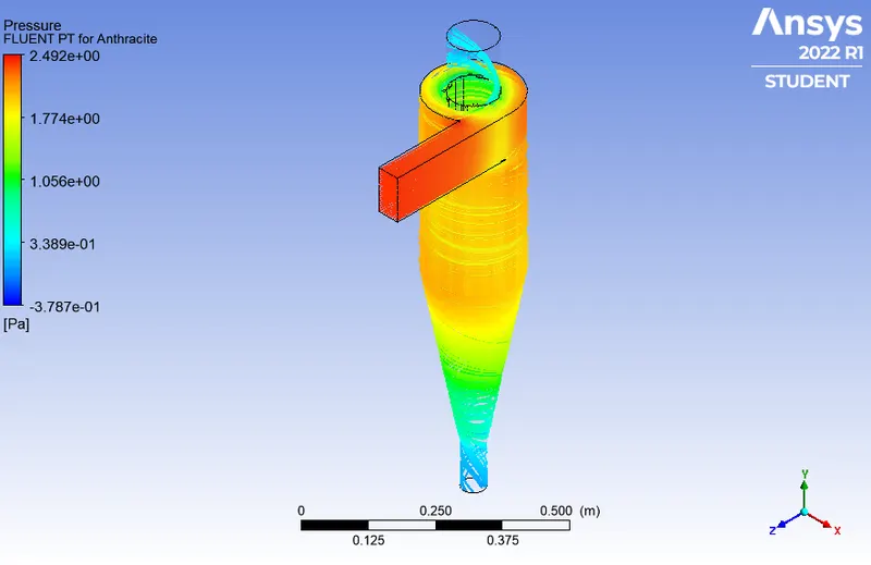
b. 2 m/s:

Residual plot:

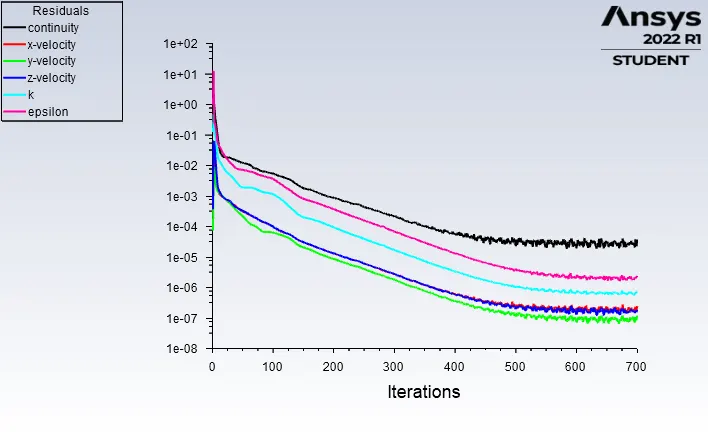
Anthracite particle contour:

Velocity contour:

Pressure contour:

c. 3 m/s:

Residual plot:

Anthracite particle contour:

Velocity contour:

Pressure contour:

d. 4 m/s:

Residual plot:

Anthracite particle contour:

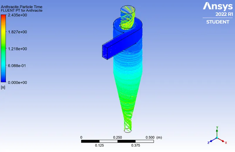
Velocity contour:

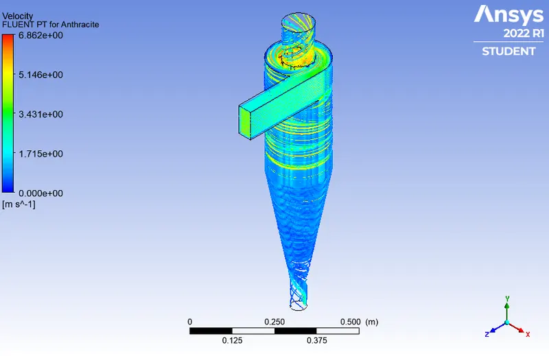
Pressure contour:

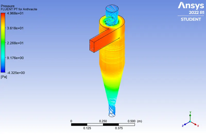
e. 5 m/s:

Residual plot:

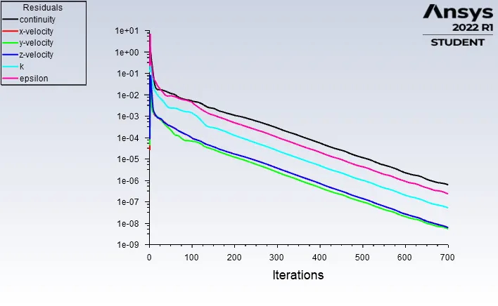
Anthracite particle contour:

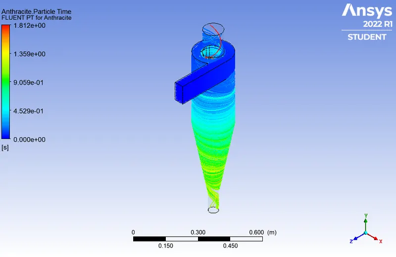
Velocity contour:

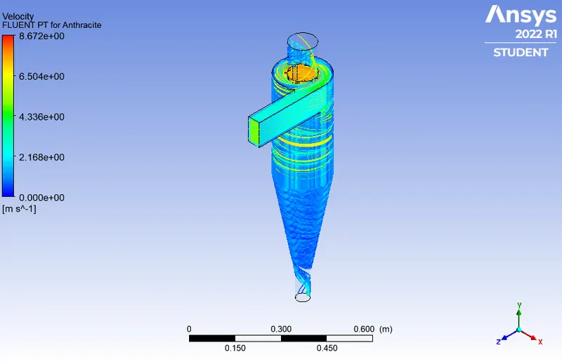
Pressure contour:

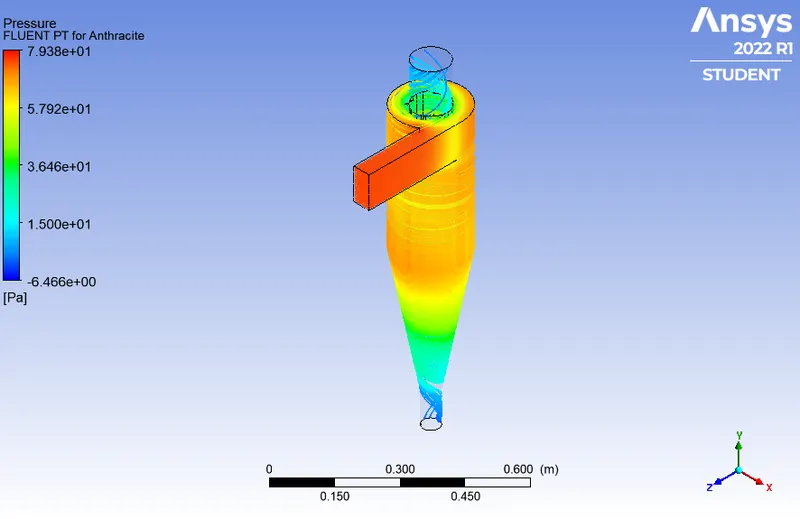
Comparison table:

1. Varying particle size with constant velocity:

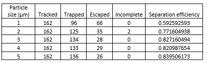
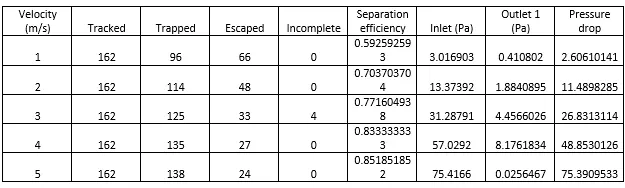
2. Varying velocity with constant particle size:

Conclusion:

From the result obtained, we can conclude that when the size of the particle starts to increase the particles getting escape through the top outlet decreases. Also, the separation efficiency increases. The velocity increase leads to the higher pressure drop. Velocity increase cause the huge difference than the size of the particle increase.