Week 6 - CHT Analysis on a Graphics card

Objective:

The aim is to perform the simulation on graphics card to analyse the conjugate heat transfer (CHT).

Conjugate Heat Transfer:

It is mathematically stated problem, describes the heat transfer between a body and a fluid flowing over or inside it as a result of the interaction of two objects. The physical processes and solutions of the governing equations are considered separately for each object in two subdomains (Body & Fluid domain). Matching conditions for these solutions at the interface provide the distributions of temperature and heat flux along the body–flow interface, eliminating the need for a heat transfer coefficient. Moreover, it may be calculated using these data.

The best way to analyse the solution for it is by using Numerical method. Set the boundary conditions for both the interface, process and converge the solution.

Application:

Conjugate heat transfer methods have become a more powerful tool for modelling and investigating nature phenomena and engineering systems in different areas ranging from aerospace and nuclear reactors to thermal goods treatment and food processing, from complex procedures in medicine to atmosphere/ocean thermal interaction in meteorology.

Heat Exchangers and Finned Surfaces (e.g., IC engine, heat sink, car radiator)

Thermal Treatment and Cooling Systems (e.g., thermal depolymerisation, cooling tower)

Simulation of Industrial Processes (e.g., inline four engine exhaust port)

Technology Processes (e.g., graphics card)

Solving & modelling approach:

• Import the graphic card geometry in space claim.
• CHT analysis on graphic card requires fins, processor and base as a separate volume because each of these solid body are made up of different material alloys.
• Set the share topology from none to share to share the information between all the volume interfaces.
• Load the geometry in meshing. Do the named selections for the inlets, outlet, wall & symmetry wall faces and mesh the geometry for baseline stuff. To analyse further, refine mesh.
• Do the necessary physics and boundary conditions setup in setup to converge the solution.
• Finally, compare the result of contour and graph plot.

Pre-processing and solver setting:

Baseline mesh:

Geometry:

Import the geometry in space claim.

Set the share topology from none to share to share the information between all the volume interfaces.

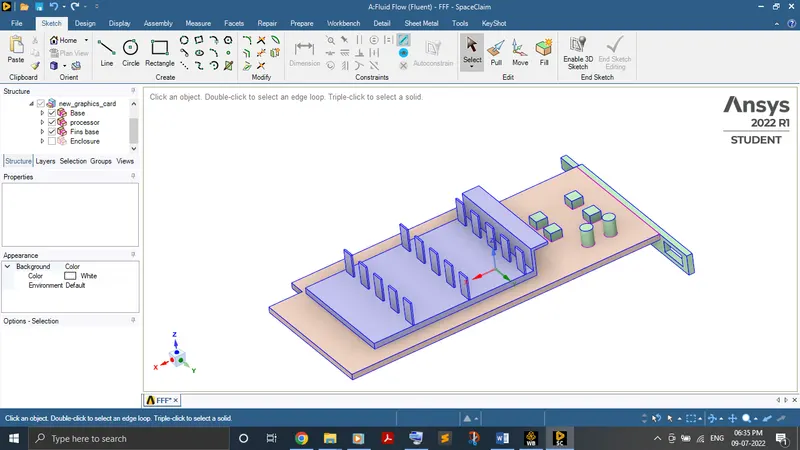
Those pink lines are the indication of sharing the information between the volumes. If we don't do this, information exchange does'nt happen and leads to poor mesh which leads to affect the result.

Meshing:

Load the geometry in meshing and do the named selections for the faces.

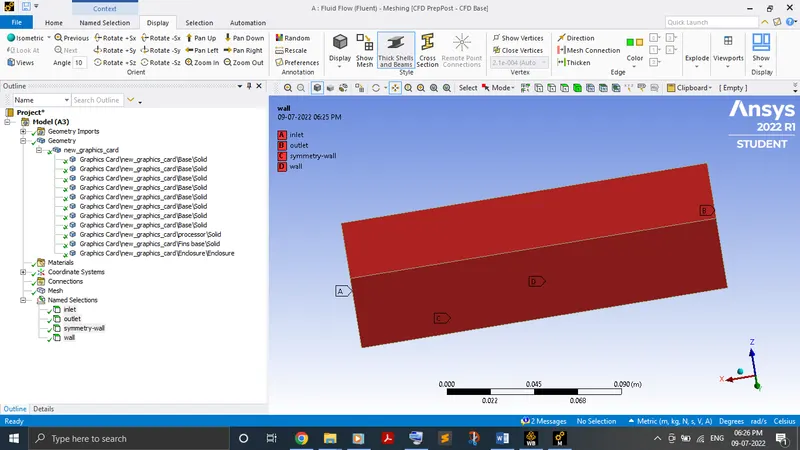
Do the baseline mesh for the geometry.

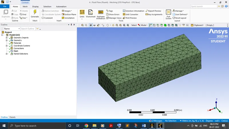
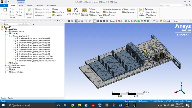
Nodes - 15722

Element - 83822

Setup:

Solver type - Steady state pressure based

Model - Energy equation, K-omega viscous turbulence model

Material - Fluid (enclosure - air), Solid (fins - aluminium, base - copper, processor - silicon)

Cell zone condition - In processor, select the source term in edit because here the processor is the only heat generated one.

Here, I considered my processor (AMD A10 7300 radeon r6) power as 19 W and the volume of the processor is 64mm.

q = P/V = 296875000 W/m²

Boundary conditions:

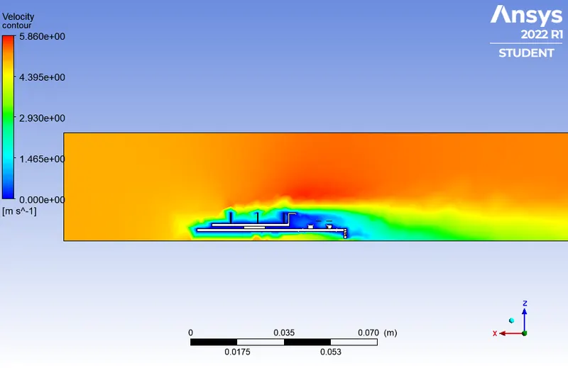
Inlet velocity - Velocity magnitude (5 m/s), Temperature (300 K)

Outlet pressure gauge - 0

Wall - coupled

Results:

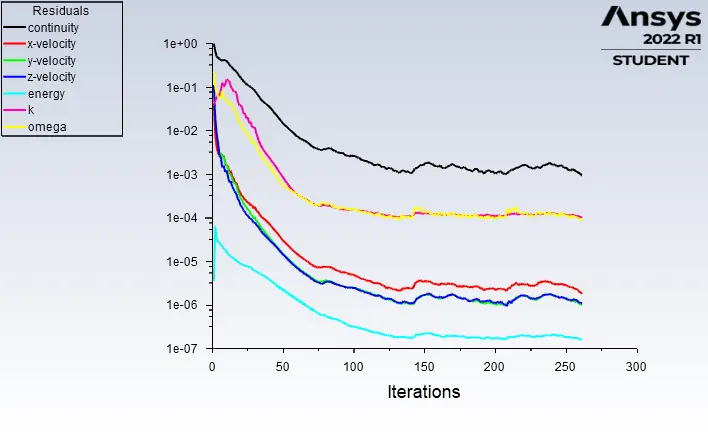
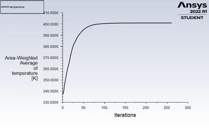
Residual plot:

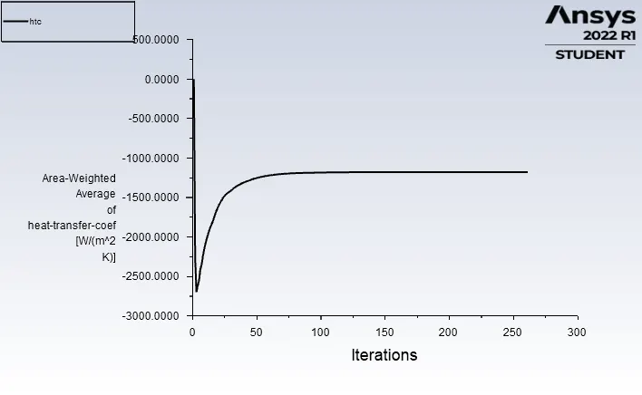
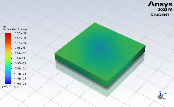
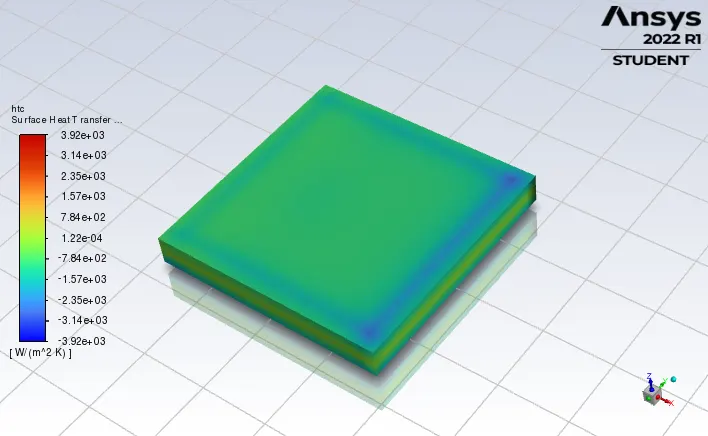
Surface heat transfer co-efficient on processor: -1177.6074 W/m²K

Plot:

Contour:

Velocity contour:

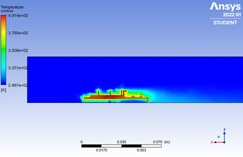
Temperature contour:

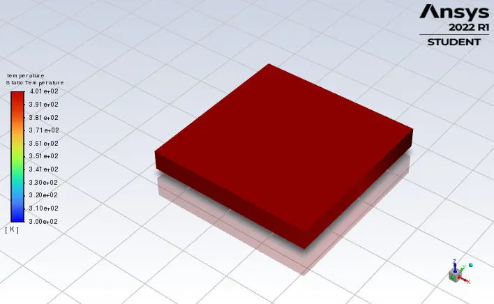
Processor:

1. Contour:

2. Plot:

Overall:

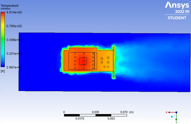
Hotspot:

Refined mesh:

Everything is similar to the baseline mesh except refining the volume of each individually and for the different result comparison tried three different velocities at inlet boundary conditions.

Mesh update:

Element size of the enclosure: 0.0018 m

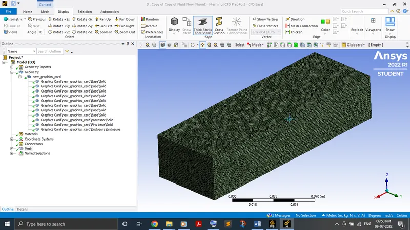
Body sizing:

Processor – 0.0005 m

Fins – 0.00075 m

Base – 0.001 m

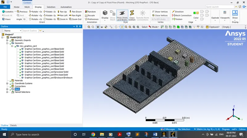
Node - 91694

Element - 498734

Setup:

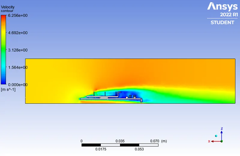
Case (a): Velocity - 5 m/s

Results:

Residual plot:

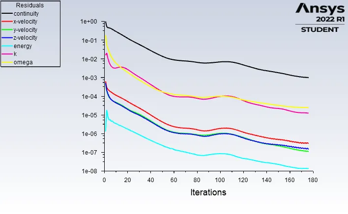
Surface heat transfer co-efficient on processor: -1358.7721 W/m²K

Plot:

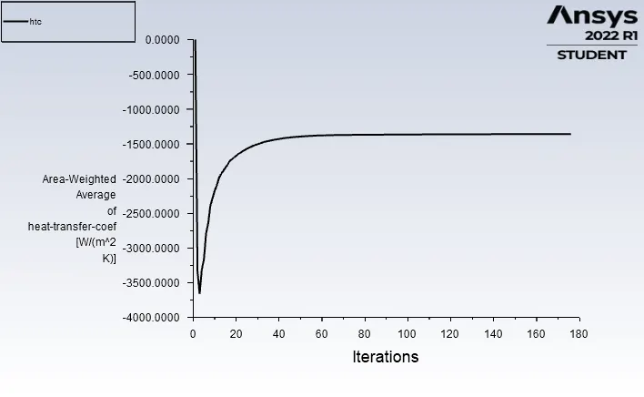
Contour:

Velocity contour:

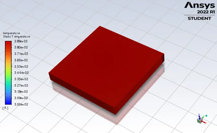
Temperature contour:

Processor:

1. Contour:

2. Plot:

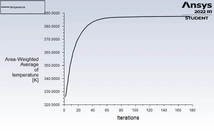
Overall:

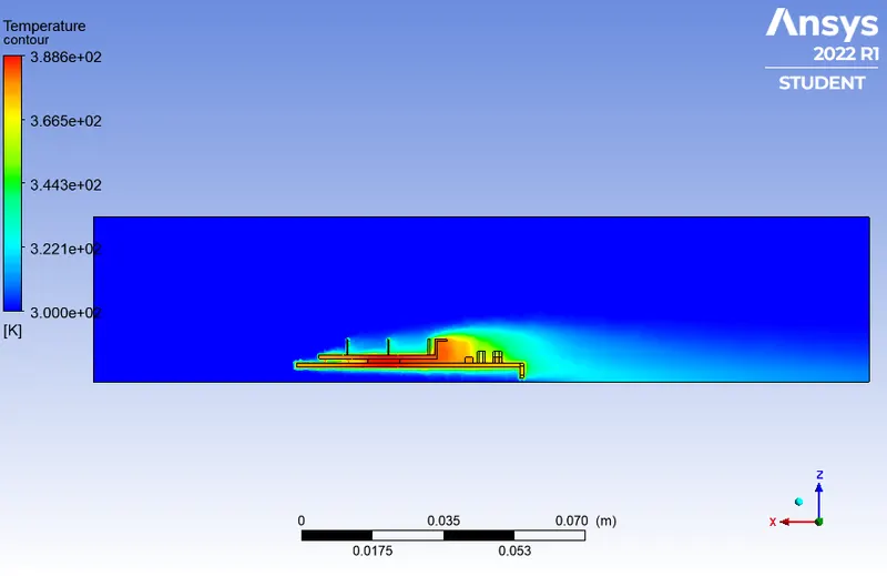
Hotspot:

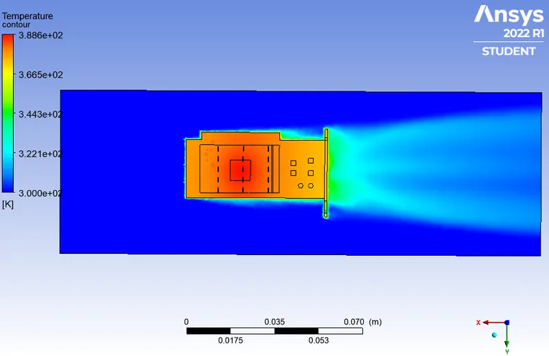
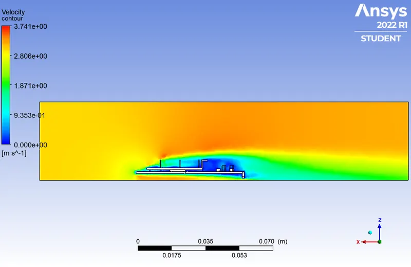
Case (b): Velocity - 3 m/s

Results:

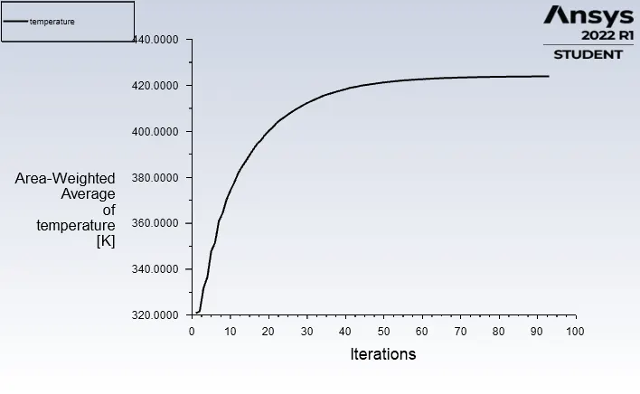
Residual plot:

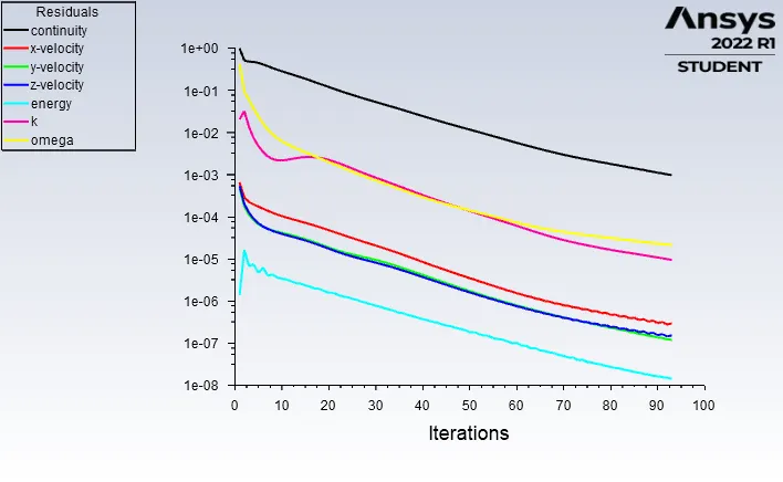
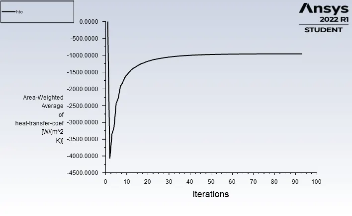
Surface heat transfer co-efficient on processor: -959.07586 W/m²K

Plot:

Contour:

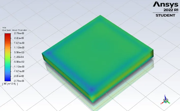
Velocity contour:

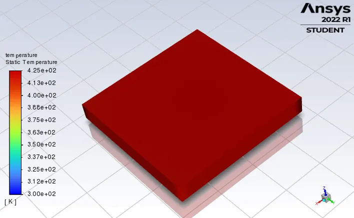
Temperature contour:

Processor:

1. Contour:

2. Plot:

Overall:

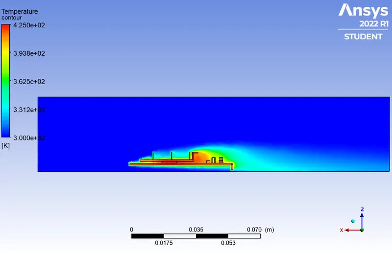
Hotspot:

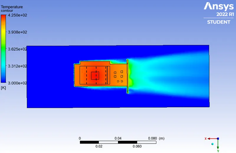
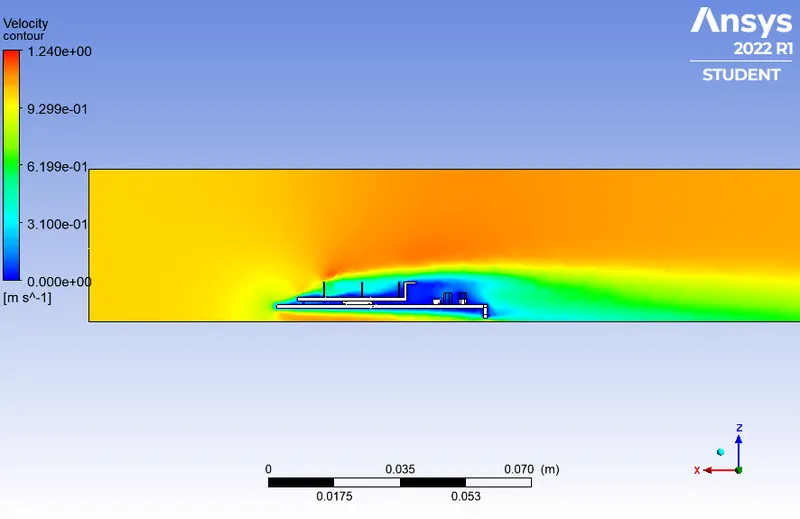
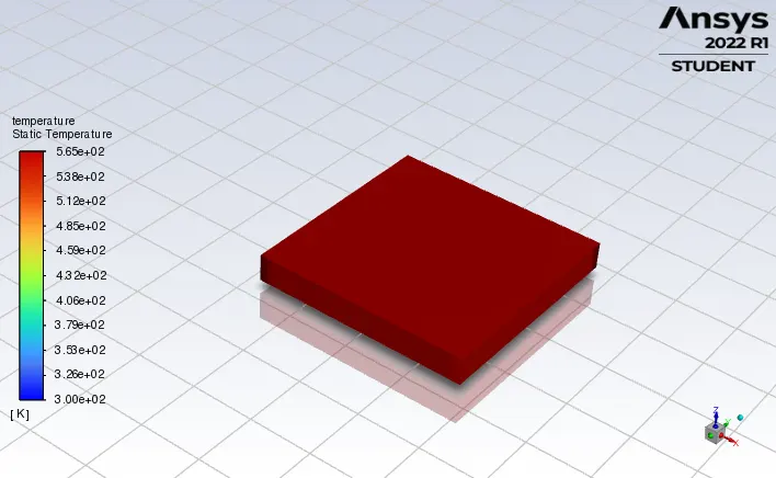
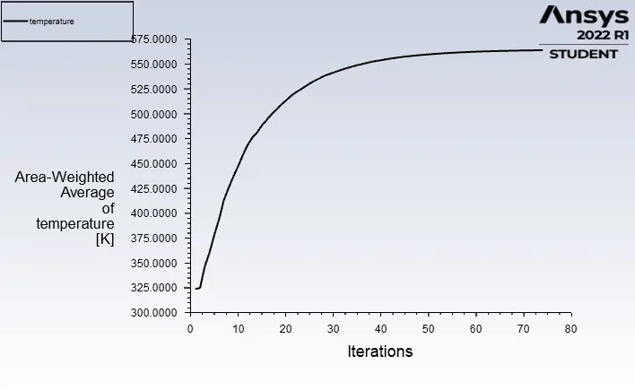
Case (c): Velocity - 1 m/s

Results:

Residual plot:

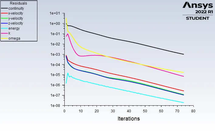
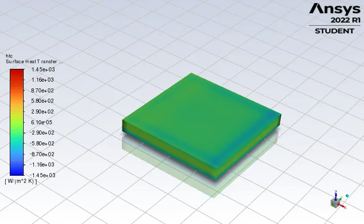
Surface heat transfer co-efficient on processor: -450.28452 W/m²K

Plot:

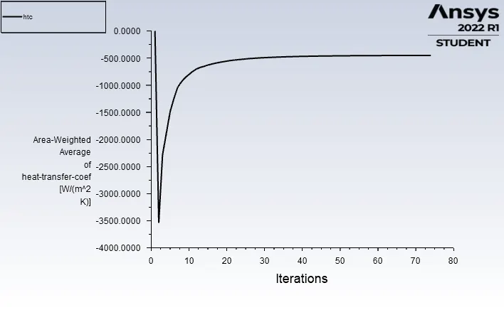
Contour:

Velocity contour:

Temperature contour:

Processor:

1. Contour:

2. Plot:

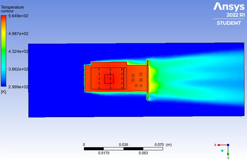
Overall:

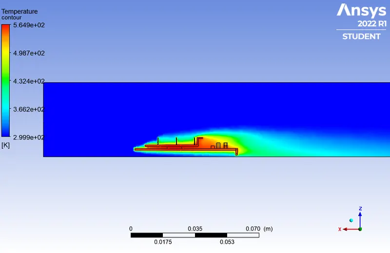
Hotspot:

Comparison:

	Baseline mesh	Refined mesh
Velocity (m/s)	5	5	3	1
Maximum temperature on the processor[K]	400.94203	387.50383	423.92021	563.83333
Maximum surface HTC on the processor (W/m2K)	-1177.6074	-1358.7721	-959.07586	-450.28452

Conclusion:

From the result obtained, we can conclude that HTC starts to increase when the velocity decreases which leads to the heat dissipation on the graphics card. So, at the same time temperature starts to decrease. This kind of mesh has done for getting the result much accurately. Simply, more you refine the mesh, the result will be much accurate. Also, solution gets converged in lesser iteration in the refined mesh than the baseline mesh. Hotspot is obtained on the processor because it's the heat conductor on graphics card. So, the other spots like fins and base seems to be the hotspots due to having contact with it. But, temperature on the graphics card can get dissipated easily by increasing velocity at the inlet. This is the convection process.