Week 4.1 - Genetic Algorithm

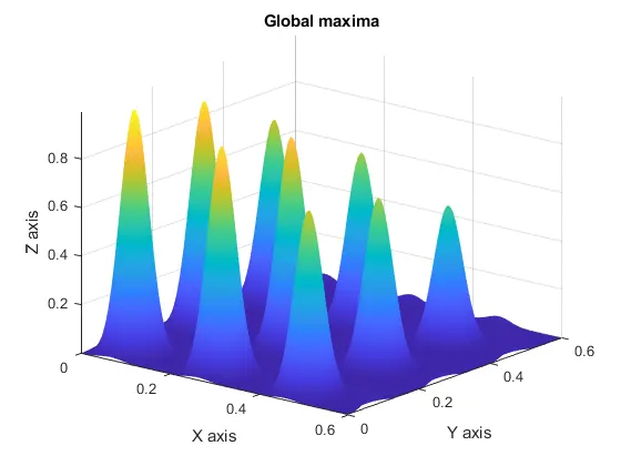
Objective: The aim is to obtain a code in MATLAB to optimise the stalagmite function and find the global maxima of the function.

Theory of ga: Genetic algorithm is a search algorithm based on the mechanics of natural selection and natural genetics. They combine the survival of the fittest among string structures with the structured yet randomized information exchange to form a search algorithm with some of the innovative flair of human search. This has been developed by “John Holland”. Goal is to abstract & rigorously explain the adaptive process of natural system and to design artificial system software that retains the important mechanism of natural systems.

(Reference - “Genetic algorithm” by David Goldberg)

A simple genetic algorithm that yields good results in many practical problems are composed of three operators:

1. Reproduction – It’s nothing but a selection process in which need to pick the fitted value to get the great result at the end.
2. Crossover – It’s nothing but a process happening between two fitted value to get the new great result.
3. Mutation – It’s nothing but a process of doing some random changes of the fitted value.

Syntex of ga: It helps to minimize the function.

x = ga (fun,nvars)

x = ga (fun,nvars,A,b)

x = ga (fun,nvars,A,b,Aeq,beq)

x = ga (fun,nvars,A,b,Aeq,beq,lb,ub)

x = ga (fun,nvars,A,b,Aeq,beq,lb,ub,nonlcon)

x = ga (fun,nvars,A,b,Aeq,beq,lb,ub,nonlcon,options)

x = ga (fun,nvars,A,b,[],[],lb,ub,nonlcon,IntCon)

x = ga (fun,nvars,A,b,[],[],lb,ub,nonlcon,IntCon,options)

x = ga (problem)

[x,fval] = ga (___)

[x,fval,exitflag,output] = ga (___)

[x,fval,exitflag,output,population,scores] = ga (___)

fun – Function name

nvars – Number of variables in function

A – Matrix for linear inequality

b – Normal vector for linear inequality

Aeq – Matrix for linear equality

beq - Normal vector for linear equality

lb – lower bound variables

ub – upper bound variables

nonlcon – Non linear constraint

IntCon – Integer constraint

options – Use optimoptions function to store the option result by taking ga result as an input

fval – Fitness value

x – Input argument

x = ga(fun,nvars) finds a local unconstrained minimum, x, to the objective function, fun. nvars is the dimension (number of design variables) of fun.

x = ga(fun,nvars,A,b) finds a local minimum x to fun, subject to the linear inequalities A*x ≤ b. ga evaluates the matrix product A*x as if x is transposed (A*x').

x = ga(fun,nvars,A,b,Aeq,beq) finds a local minimum x to fun, subject to the linear equalities Aeq*x = beq and A*x ≤ b. (Set A=[] and b=[] if no linear inequalities exist.) ga evaluates the matrix product Aeq*x as if x is transposed (Aeq*x').

x = ga(fun,nvars,A,b,Aeq,beq,lb,ub) defines a set of lower and upper bounds on the design variables, x, so that a solution is found in the range lb ≤ x ≤ ub. (Set Aeq=[] and beq=[] if no linear equalities exist.)

x = ga(fun,nvars,A,b,Aeq,beq,lb,ub,nonlcon) subjects the minimization to the constraints defined in nonlcon. The function nonlcon accepts x and returns vectors C and Ceq, representing the nonlinear inequalities and equalities respectively. ga minimizes the fun such that C(x) ≤ 0 and Ceq(x) = 0. (Set lb=[] and ub=[] if no bounds exist.)

x = ga(fun,nvars,A,b,Aeq,beq,lb,ub,nonlcon,options) minimizes with the default optimization parameters replaced by values in options. (Set nonlcon=[] if no nonlinear constraints exist.) Create options using optimoptions.

x = ga(fun,nvars,A,b,[],[],lb,ub,nonlcon,IntCon) or x = ga(fun,nvars,A,b,[],[],lb,ub,nonlcon,IntCon,options) requires that the variables listed in IntCon take integer values. When there are integer constraints, ga does not accept linear or nonlinear equality constraints, only inequality constraints.

x = ga(problem) finds the minimum for problem, a structure described in problem.

[x,fval] = ga(___), for any previous input arguments, also returns fval, the value of the fitness function at x.

[x,fval,exitflag,output] = ga(___) also returns exitflag, an integer identifying the reason the algorithm terminated, and output, a structure that contains output from each generation and other information about the performance of the algorithm.

[x,fval,exitflag,output,population,scores] = ga(___) also returns a matrix population, whose rows are the final population, and a vector scores, the scores of the final population.

Code:

1) For Global maxima

% Global maxima

% defining our search space
% one dimensional array
x = linspace(0,0.6,150);
y = linspace(0,0.6,150);

% creating 2D array
[xx yy] = meshgrid(x,y);

% evaluating the stalagmite function
for i = 1:length(xx)
    for j = 1:length(yy)
        inputs(1) = xx(i,j);
        inputs(2) = yy(i,j);
        f(i,j) = get_stalagmite(inputs);
    end
end

surfc(xx,yy,f)
shading interp
title('Global maxima')
xlabel('X axis')
ylabel('Y axis')
zlabel('Z axis')
[inputs, fval] = ga(@get_stalagmite,2);

function [f] = get_stalagmite(inputs)
x = inputs(1);
y = inputs(2);
f_1x = (sin(5.1*pi*x + 0.5)).^6;
f_1y = (sin(5.1*pi*y + 0.5)).^6;
f_2x = exp(-4*log10(2)*((x-0.0667).^2/0.64));
f_2y = exp(-4*log10(2)*((y-0.0667).^2/0.64));
f = ((f_1x)*(f_1y)*(f_2x)*(f_2y));
end

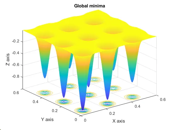
2) Minima

clear all
close all
clc

% Global minima

% defining our search space
% one dimensional array
x = linspace(0,0.6,150);
y = linspace(0,0.6,150);
num_cases = 50;

% creating 2D array
[xx yy] = meshgrid(x,y);

% evaluating the stalagmite function
for i = 1:length(xx)
    for j = 1:length(yy)
        inputs(1) = xx(i,j);
        inputs(2) = yy(i,j);
        f(i,j) = get_stalagmite(inputs);
    end
end

surfc(xx,yy,f)
shading interp
title('Global minima')
xlabel('X axis')
ylabel('Y axis')
zlabel('Z axis')
[inputs, fval] = ga(@get_stalagmite,2);

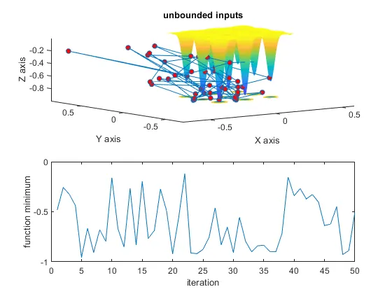
% study 1 - statical behaviour
for i = 1:num_cases
    [inputs, fopt(i)] = ga(@get_stalagmite, 2);
        xopt(i) = inputs(1);
        yopt(i) = inputs(2);
end

figure(2)
subplot(2,1,1)
hold on
surfc(xx,yy,f)
shading interp
plot3(xopt,yopt,fopt,'marker','o','markersize',5,'markerfacecolor','r')
title('unbounded inputs')
xlabel('X axis')
ylabel('Y axis')
zlabel('Z axis')
subplot(2,1,2)
plot(fopt)
xlabel('iteration')
ylabel('function minimum')

tic
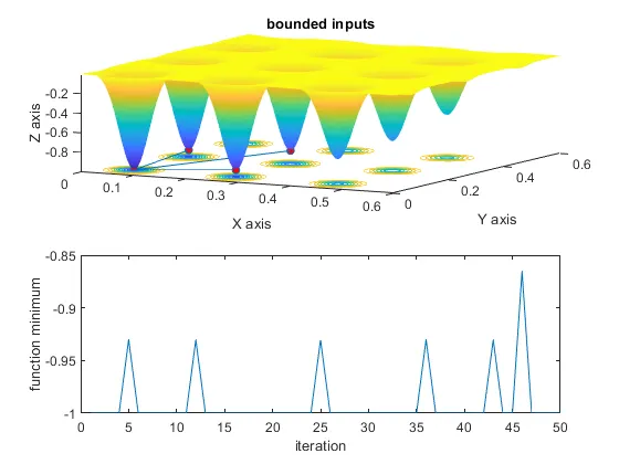
% study 2 - statical behaviour with upper & lower bound
for i = 1:num_cases
    [inputs, fopt(i)] = ga(@get_stalagmite,2,[],[],[],[],[0;0],[0.6;0.6]);
        xopt(i) = inputs(1);
        yopt(i) = inputs(2);
end
study2_time = toc

figure(3)
subplot(2,1,1)
hold on
surfc(xx,yy,f)
shading interp
plot3(xopt,yopt,fopt,'marker','o','markersize',5,'markerfacecolor','r')
title('bounded inputs')
xlabel('X axis')
ylabel('Y axis')
zlabel('Z axis')
subplot(2,1,2)
plot(fopt)
xlabel('iteration')
ylabel('function minimum')

% study 3 - increasing ga iteration
options = optimoptions('ga');
options = optimoptions(options,'populationsize',150);

tic
for i = 1:num_cases
    [inputs, fopt(i)] = ga(@get_stalagmite,2,[],[],[],[],[0;0],[0.6;0.6],[],[],options);
        xopt(i) = inputs(1);
        yopt(i) = inputs(2);
end
study3_time = toc

figure(4)
subplot(2,1,1)
hold on
surfc(xx,yy,f)
shading interp
plot3(xopt,yopt,fopt,'marker','o','markersize',5,'markerfacecolor','r')
title('bounded inputs')
xlabel('X axis')
ylabel('Y axis')
zlabel('Z axis')
subplot(2,1,2)
plot(fopt)
xlabel('iteration')
ylabel('function minimum')

function [f] = get_stalagmite(inputs)
x = inputs(1);
y = inputs(2);
f_1x = (sin(5.1*pi*x + 0.5)).^6;
f_1y = (sin(5.1*pi*y + 0.5)).^6;
f_2x = exp(-4*log10(2)*((x-0.0667).^2/0.64));
f_2y = exp(-4*log10(2)*((y-0.0667).^2/0.64));
f = -((f_1x)*(f_1y)*(f_2x)*(f_2y));
end

The purpose of using tic toc command is to check how long the iteration takes to gives the output. It gives the time of the iteration in the command window.

Explanation:

Global maxima: Initially, defined search space(x&y) in 1D array and used meshgrid command to set the 2D array for XX & YY. Then, processed stalagmite function to store in array “f” for the assigned functional equation with the variables of 2 and storing the variable values within the function as an input(1)(for x) & input(2)(for y) which means it’s a row vector. First x takes 1 column value & y takes 2 column value. Finally, for getting multiple results I used for loop by giving condition to the “I” & “j” and stored value of XX & YY for each and every (I,j) in the inputs to get the output “f” for the same. For the great plotting result, used some commands like title, lables for axis, surfc(for 3D plotting) etc.. “Shading interp” command helps to get the smooth result. Without this, result get a meshgrid automatically. When we use the ga inbuilt algorithm, we need to give in the input in the format of function name & no. of functional variables for the input argument x to return the fval and store it as on output.

Global minima: It’s similar to the process of maxima except the alternation of the sign in the functional equation. Every study condition’s used ga format has its description in the syntax of ga.

Result:

1)

2)