Week 1- Mixing Tee
Objective:
The aim is to that we have created two versions of the mixing tee. One of them is longer than the other.
The job is to set up steady-state simulations to compare the mixing effectiveness when hot inlet temperature is 360C & the Cold inlet is at 190C.
Use the k-epsilon and k-omega SST model for the first case and based on your judgment use the more suitable model for further cases.
- Case 1
- Short mixing tee with a hot inlet velocity of 3m/s.
- Momentum ratio of 2, 4.
- Case 2
- Long mixing tee with a hot inlet velocity of 3m/s.
- Momentum ratio of 2, 4.
These given conditions are going to perform using Ansys fluent.
Mixing tee:
Mixing Tees utilizes a specifically engineered internal geometry to efficiently mix two fluid streams into one combined stream. Mixing Tees are ideal for analytical gradient HPLC. These mixing tees are specifically designed for high pressure applications.
Ansys fluent workflow:
Ansys workbench:
Initially, launch the Ansys workbench and create a new fluid flow analysis system by double clicking the “Fluid flow (fluent)” option which is under “Analytical systems” in the toolbox.
Geometry:
For a geometry we need to do fluid flow analysis, either we create the geometry or import the appropriate geometry here.
Mesh:
For the created or imported geometry, we need to generate a computational mesh throughout the flow volume. This can be done here with the help of Meshing application of Ansys.
Setup:
Setting up a necessary case conditions here for the CFD analysis using Ansys fluent.
Solution:
Solution initialization and run calculation can perform to visualize the required results in console (iteration result) and graphic window (plot results).
Results:
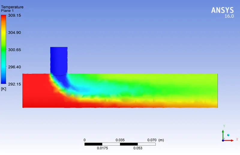
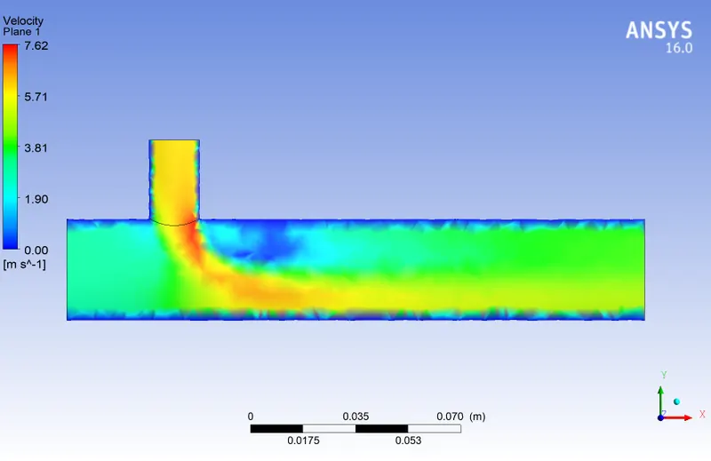
Post processing can perform here like a simple evaluation of the velocity and temperature contours on the symmetry plane.
Short tee:
Geometry setup:
Import the geometry of step file to the Ansys space claim.
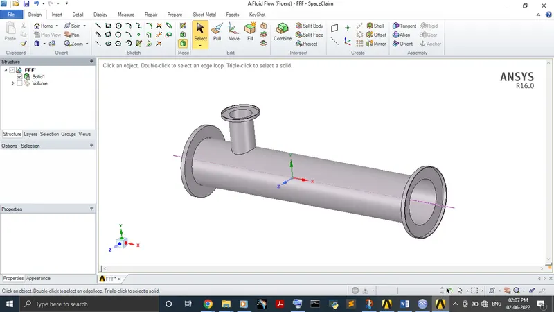
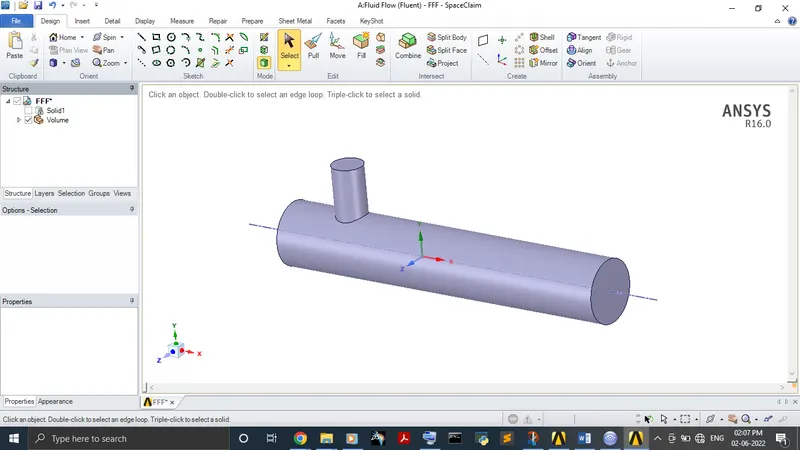
Here, keep only the volume through which the fluid going to flow. Other than the fluid flow doesn’t takes place solid parts should be subtract using volume extract. Finally, suppress the physics for solid which is shown under structure because of not to take part in future process like meshing.
Mesh generation:
Here, mesh the geometry as of the requirement by choosing it in the sizing from the details of mesh.
The faces can be named by using named selections option.
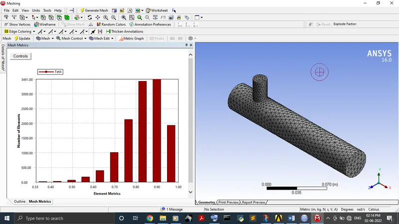
The mesh quality can check by choosing element quality in mesh metric which comes under quality in details of mesh.
The element quality should be greater or equal to 0.05. In our case, it’s around 0.35. It’s okay to proceed further.
Setup & Solution:
Case 1 (a):
- Short mixing tee with a hot inlet velocity of 3m/s.
- Momentum ratio of 2
|
K Epsilon |
K omega |
|
|
Solver Type |
Pressure based |
Pressure based |
|
Solver Velocity formulation |
Absolute |
Absolute |
|
Solver Time |
Steady |
Steady |
|
Viscous Model |
Realizable, K-Epsilon, Standard Wall functions |
SST, K-Omega model |
|
Materials |
Air |
Air |
|
Cell zones conditions |
Air |
Air |
|
Boundary conditions |
· Inlet_x Velocity (3 m/s) Temperature (36°C) · Inlet_y Velocity (6 m/s) Temperature (19°C) · Outlet (Pressure outlet) Gauge pressure(0) · Walls - Stationary |
· Inlet_x Velocity (3 m/s) Temperature (36°C) · Inlet_y Velocity (6 m/s) Temperature (19°C) · Outlet (Pressure outlet) Gauge pressure(0) · Walls - Stationary |
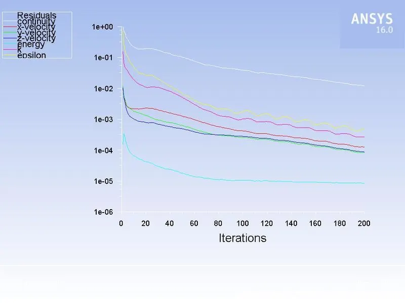
Hybrid scheme is used for initialize the solution and run calculation by setting the number of iterations.
Results:
K-Epsilon model:
Residual plot:
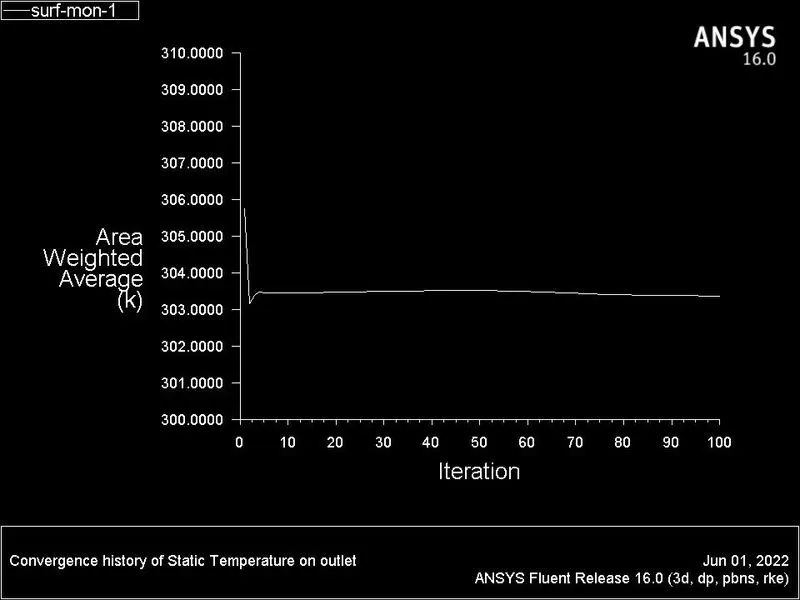
Area weighted average:
Standard deviation:
Contour plot:
Temperature:
Velocity:
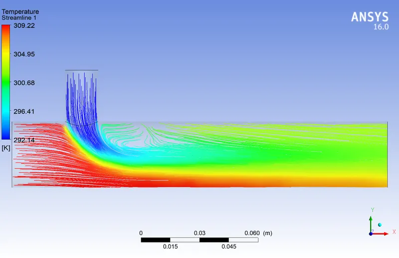
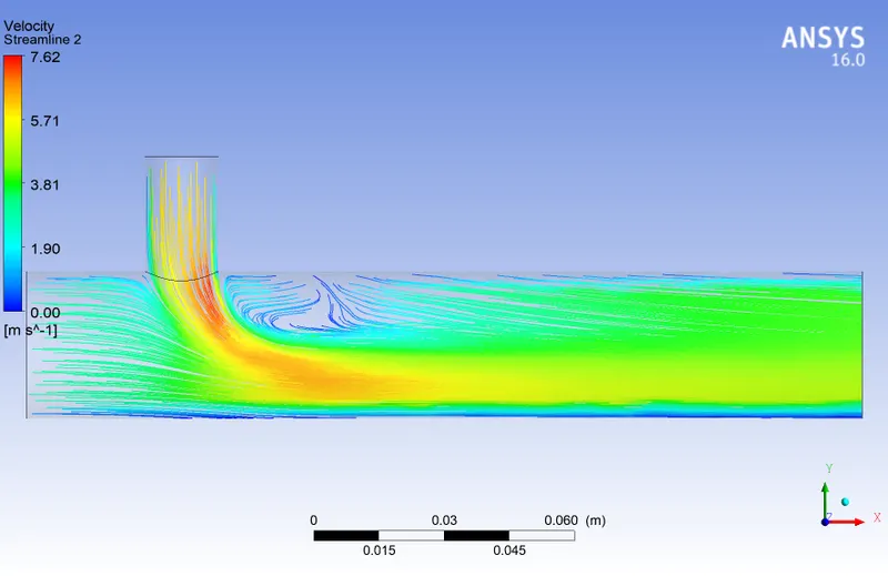
Streamline plot:
Temperature:
Velocity:
K-Omega model:
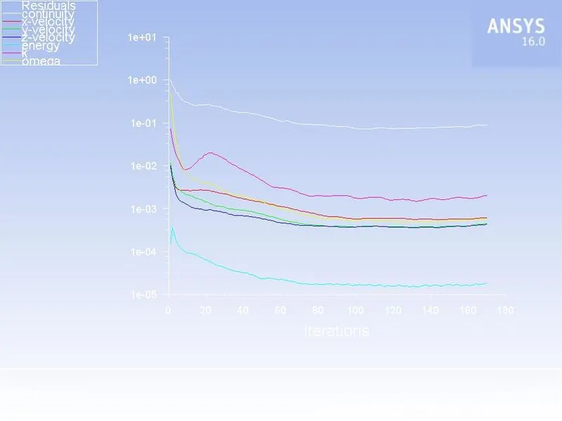
Residual plot:
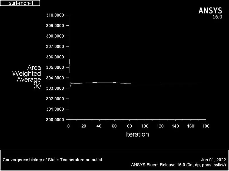
Area weighted average:
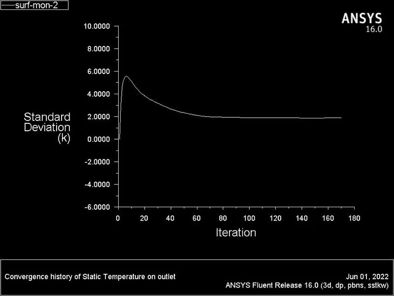
Standard deviation:
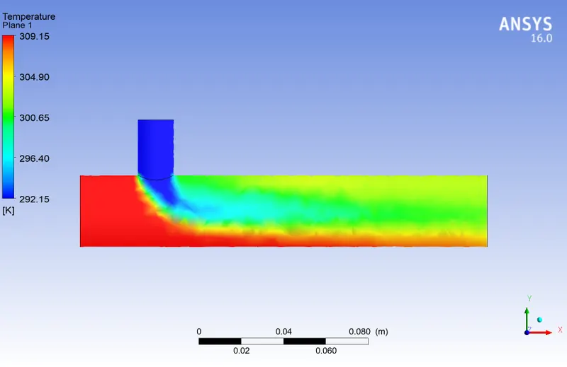
Contour plot:
Temperature:
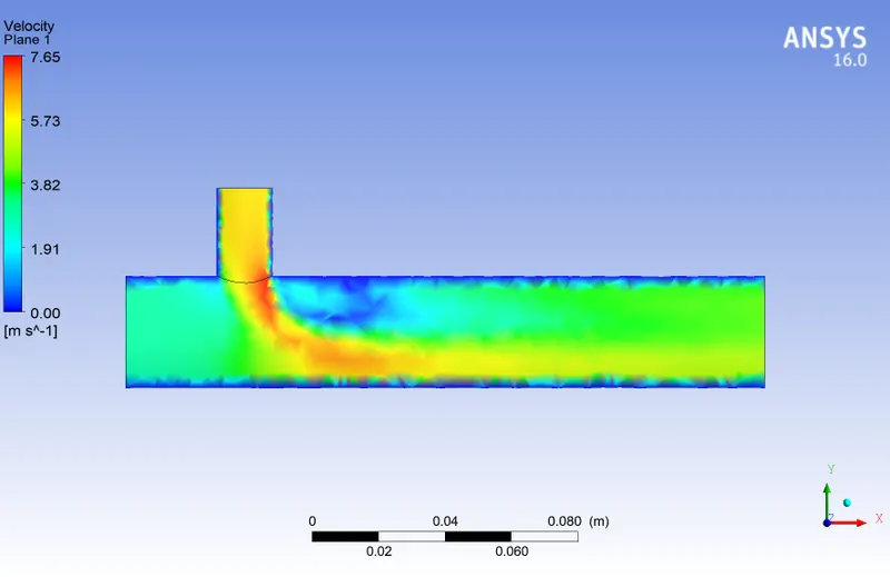
Velocity:
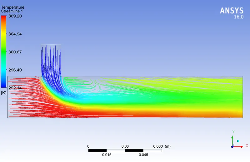
Streamline plot:
Temperature:
Velocity:
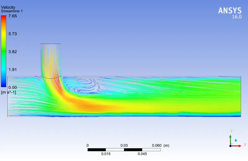
Comparison:
|
K Epsilon |
K omega |
|
|
Average outlet temperature[K] |
303.3644 |
303.3704 |
|
Cell count |
12564 |
12564 |
|
No. of iteration |
100 |
170 |
Case 1 (b):
- Short mixing tee with a hot inlet velocity of 3m/s.
- Momentum ratio of 4
For this case, only one change we should do that's the momentum ratio i.e., 4 (Cold air inlet velocity is 12 m/s). Other than this, geometry, mesh, setup are similar as previous case.
Results:
K-Epsilon model:
Residual plot:
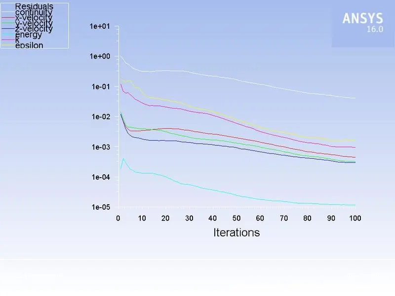
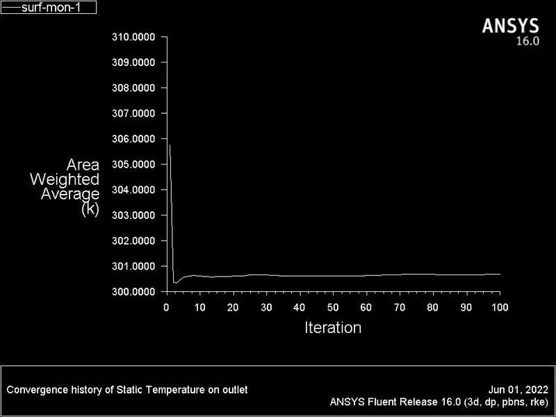
Area weighted average:
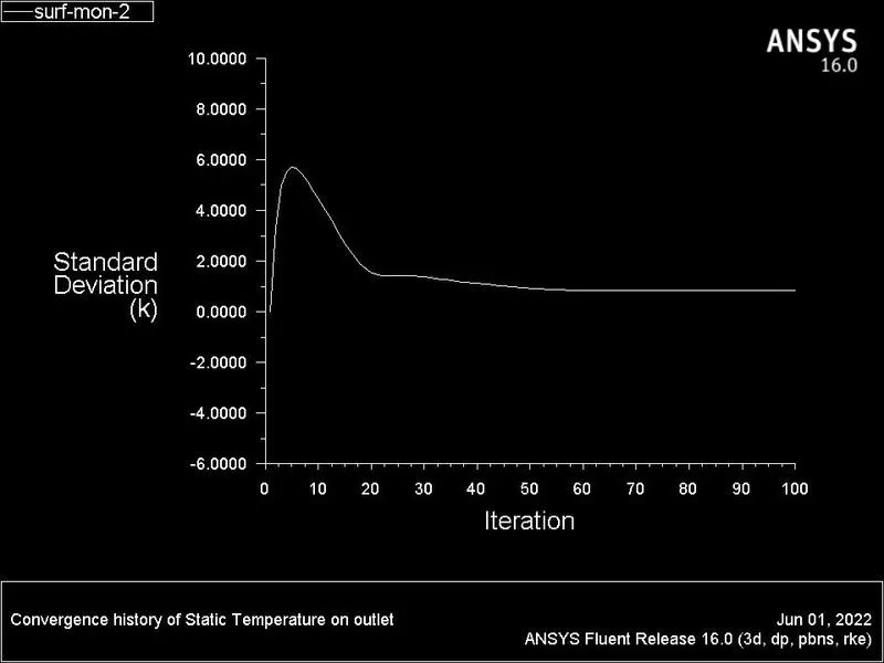
Standard deviation:
Contour plot:
Temperature:
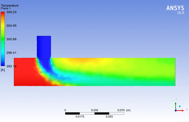
Velocity:
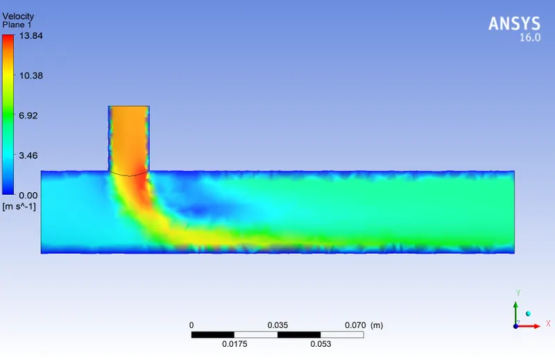
Streamline plot:
Temperature:
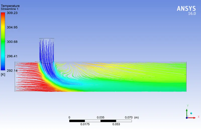
Velocity:
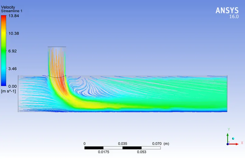
K-Omega model:
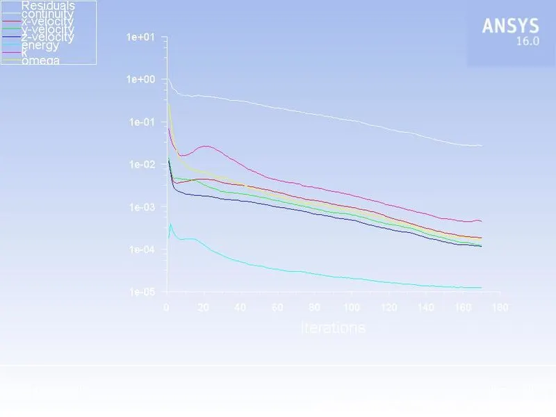
Residual plot:
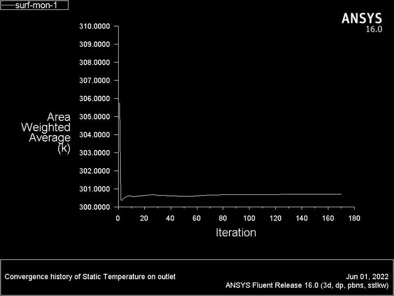
Area weighted average:
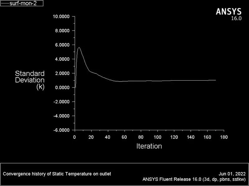
Standard deviation:
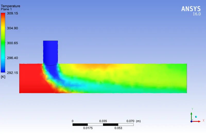
Contour plot:
Temperature:
Velocity:
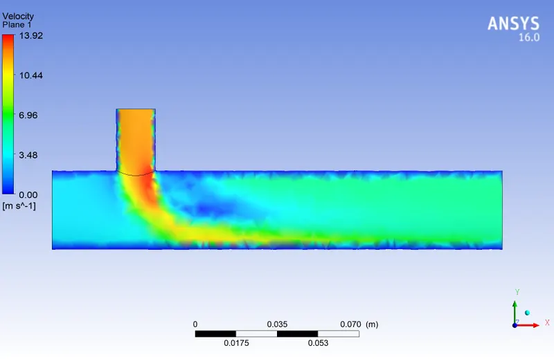
Streamline plot:
Temperature:
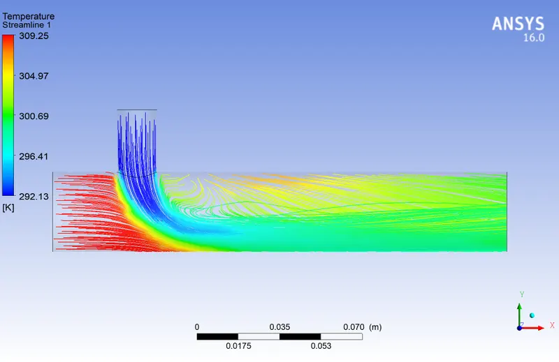
Velocity:
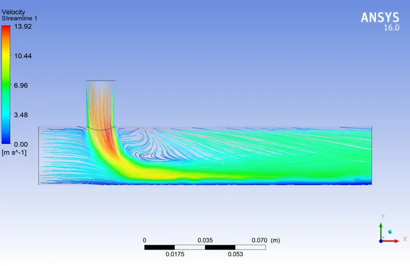
Comparison:
|
K Epsilon |
K omega |
|
|
Average outlet temperature[K] |
300.6705 |
300.6914 |
|
Cell count |
12564 |
12564 |
|
No. of iteration |
100 |
170 |
Conclusion:
Average outlet temperature:
Both viscous models gives nearly the similar results.
No. of iteration:
K-Epsilon model took much iteration to converge the solution than K-Omega model.
Standard deviation:
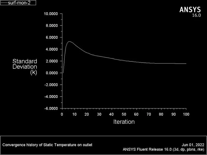
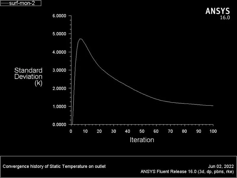
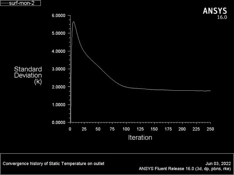
K-Epsilon model shows the result of standard deviation less when compared to K-Omega model. So, fluid mixing efficiency is better in K-Epsilon.
From the result obtained, we can conclude that K-Epsilon turbulence model gives the result accurately in less number of iterations itself. So, we consider K-Epsilon model to approach the result for next case.
Long tee:
Geometry setup:
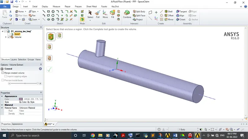
Import the geometry of step file to the Ansys space claim.
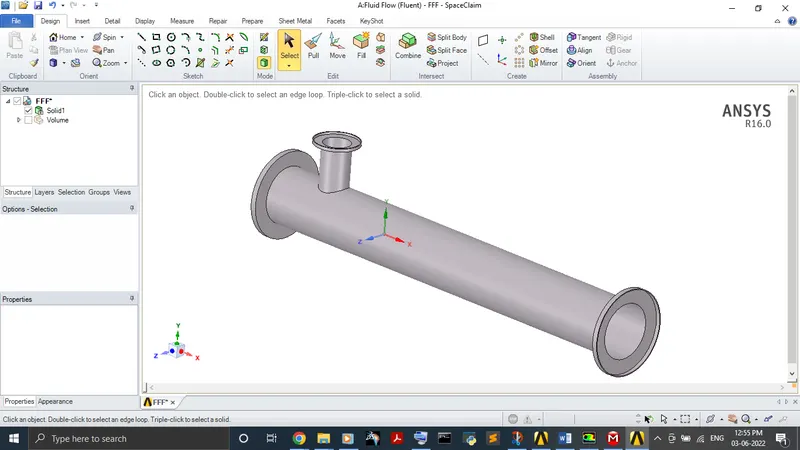
Here, keep only the volume through which the fluid going to flow. Other than the fluid flow doesn’t takes place solid parts should be subtract using volume extract. Finally, suppress the physics for solid which is shown under structure because of not to take part in future process like meshing.
Mesh generation:
Here, mesh the geometry as of the requirement by choosing it in the sizing from the details of mesh.
The faces can be named by using named selections option.
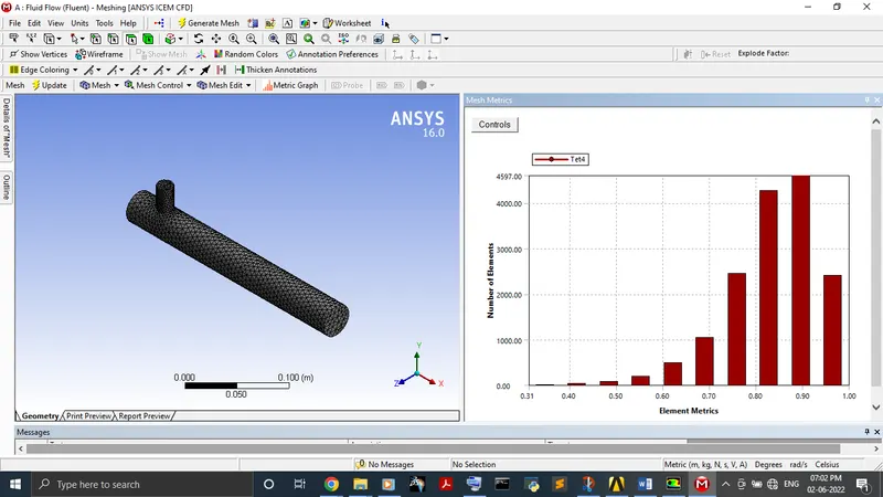
The mesh quality can check by choosing element quality in mesh metric which comes under quality in details of mesh.
The element quality should be greater or equal to 0.05.
Setup & Solution:
Case 2 (a):
- Long mixing tee with a hot inlet velocity of 3m/s.
- Momentum ratio of 2
|
K Epsilon |
|
|
Solver Type |
Pressure based |
|
Solver Velocity formulation |
Absolute |
|
Solver Time |
Steady |
|
Viscous Model |
Realizable, K-Epsilon, Standard Wall functions |
|
Materials |
Air |
|
Cell zones conditions |
Air |
|
Boundary conditions |
· Inlet_x Velocity (3 m/s) Temperature (36°C) · Inlet_y Velocity (6 m/s) Temperature (19°C) · Outlet (Pressure outlet) Gauge pressure(0) · Walls - Stationary |
Hybrid scheme is used for initialize the solution and run calculation by setting the number of iterations.
Results:
K-Epsilon model:
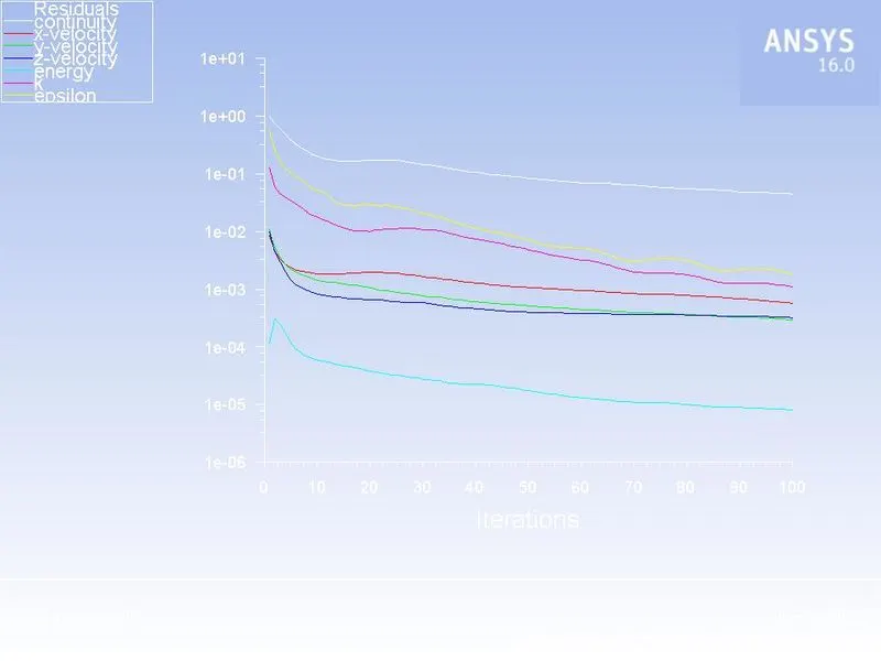
Residual plot:
Area weighted average:
Standard deviation:
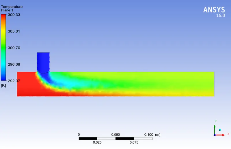
Contour plot:
Temperature:
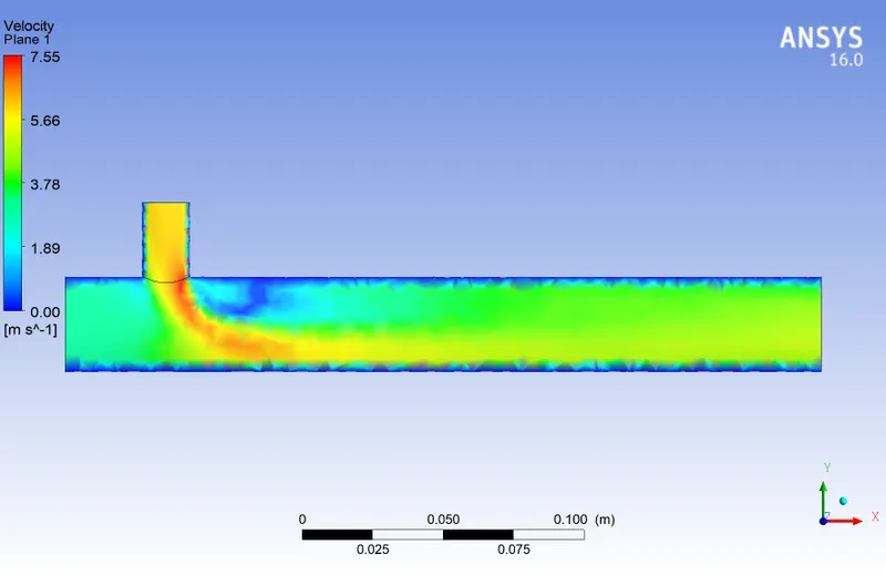
Velocity:
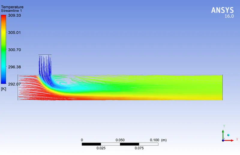
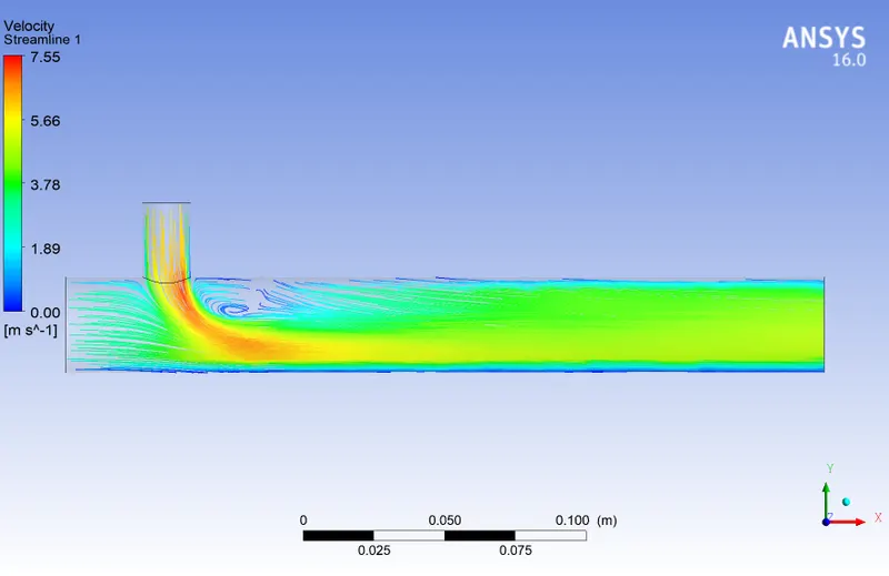
Streamline plot:
Temperature:
Velocity:
Case 2 (b):
- Long mixing tee with a hot inlet velocity of 3m/s.
- Momentum ratio of 4
|
K Epsilon |
|
|
Solver Type |
Pressure based |
|
Solver Velocity formulation |
Absolute |
|
Solver Time |
Steady |
|
Viscous Model |
Realizable, K-Epsilon, Standard Wall functions |
|
Materials |
Air |
|
Cell zones conditions |
Air |
|
Boundary conditions |
· Inlet_x Velocity (3 m/s) Temperature (36°C) · Inlet_y Velocity (12 m/s) Temperature (19°C) · Outlet (Pressure outlet) Gauge pressure(0) · Walls - Stationary |
Results:
K-Epsilon model:
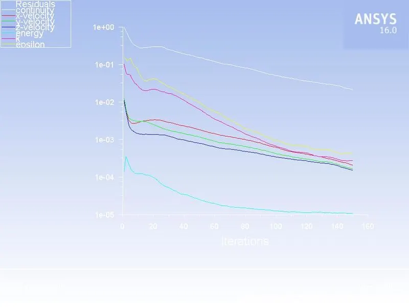
Residual plot:
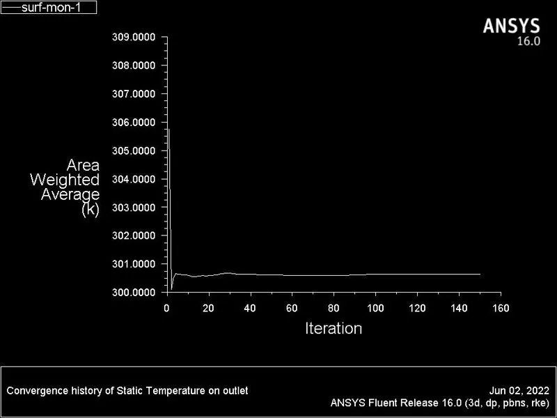
Area weighted average:
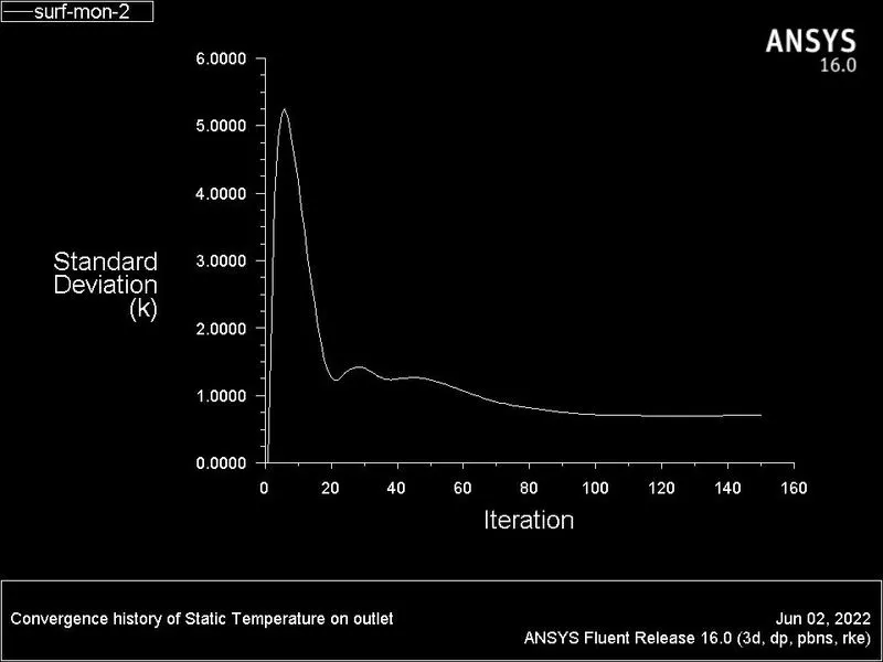
Standard deviation:
Contour plot:
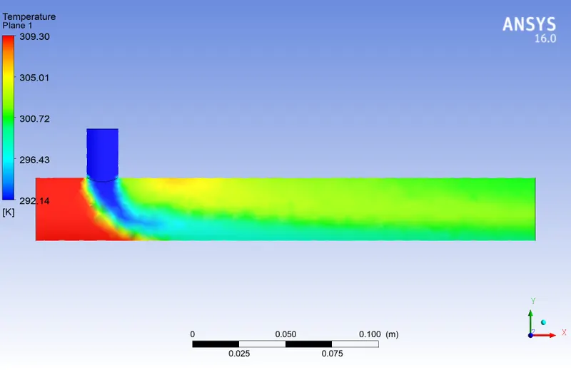
Temperature:
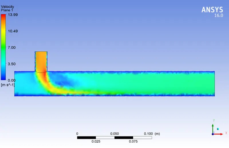
Velocity:
Streamline plot:
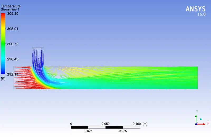
Temperature:
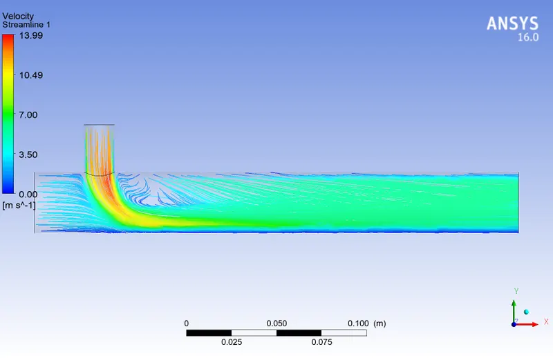
Velocity:
Comparison:
|
Momentum ratio |
2 |
4 |
|
Average outlet temperature[K] |
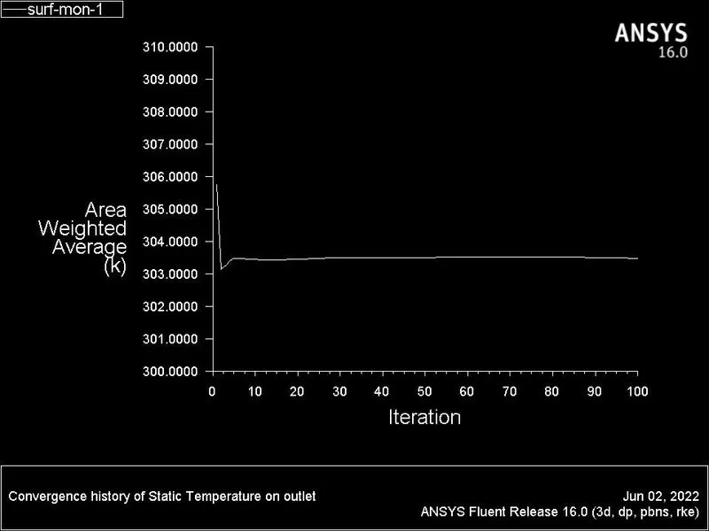
303.4853 |
300.635 |
|
Cell count |
15487 |
15487 |
|
No. of iteration |
100 |
150 |
Conclusion:
Average outlet temperature:
When the momentum ratio increases, the average outlet temperature decreases. So, it's important that cold air inlet velocity should increase to decrease the outlet temperature.
No. of iteration:
Long tee took more number of iteration to converge the solution than the short tee.
From the result obtained, we can conclude that higher the momentum ratio, mixing efficiency will be high. Long tee doesn't produce much more efficient result when compared to short tee. The results are similar only. So, length doesn't giving the effective result. But, long tee took more time and iterations to converge the solution. So, it's better to use short tee to get the efficient result in shorter time. For grid test, taken short tee to perform.
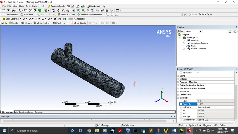
Grid Independent test:
Short tee:
Results:
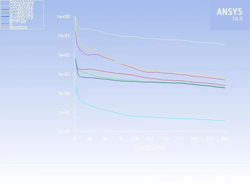
K-Epsilon model:
Residual plot:
Area weighted average:
Standard deviation:
Comparison:
|
Case 1 (a) K Epsilon model |
Grid independent test |
|
|
Average outlet temperature[K] |
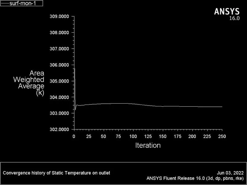
303.3644 |
303.40791 |
|
Cell count |
12564 |
41072 |
|
No. of iteration |
100 |
250 |
Conclusion:
More the mesh is fine, it starts to approach providing the result more accurate.