Week 5 - Rayleigh Taylor Instability

Objectives:

1. What are some practical CFD models that have been based on the mathematical analysis of Rayleigh Taylor waves? In your own words, explain how these mathematical models have been adapted for CFD calculations.
2. Perform the Rayleigh Taylor instability simulation for 2 different mesh sizes with the base mesh being 0.5 mm. Compare the results by showing the animations( Attach them from your google drive). Observe the differences in the animation and explain the effect of mesh size on simulation. Also, explain why a steady-state approach might not be suitable for these types of simulation.[ Choose Air and Water for this simulation]
3. Run one more simulation with water and user-defined material(density = 400 kg/m³, viscosity = 0.001 kg/m-s) for refined mesh.
4. Define the Atwood Number. Find out the Atwood number for both the cases and explain how the variation in Atwood number in the above two cases affects the behavior of the instability.

Rayleigh–Taylor instability:

The Rayleigh–Taylor instability or RT instability is an instability of an interface between two fluids of different densities which occurs when the lighter fluid is pushing the heavier fluid. Examples include the behaviour of water suspended above oil in the gravity of Earth, mushroom clouds like those from volcanic eruptions and atmospheric nuclear explosions, supernova explosions in which expanding core gas is accelerated into denser shell gas, instabilities in plasma fusion reactors and inertial confinement fusion.

Saffman–Taylor instability:

The Saffman–Taylor instability, also known as viscous fingering, is the formation of patterns in a morphologically unstable interface between two fluids in a porous medium. This situation is most often encountered during drainage processes through media such as soils. It occurs when a less viscous fluid is injected, displacing a more viscous fluid; in the inverse situation, with the more viscous displacing the other, the interface is stable and no instability is seen. In the rectangular configuration the system evolves until a single finger forms, whilst in the radial configuration the pattern grows forming fingers by successive tip-splitting.

Most experimental research on viscous fingering has been performed on Hele-Shaw cells, which consist of two closely spaced, parallel sheets of glass containing a viscous fluid. The two most common set-ups are the channel configuration, in which the less viscous fluid is injected at one end of the channel, and the radial configuration, in which the less viscous fluid is injected at the centre of the cell. Instabilities analogous to viscous fingering can also be self-generated in biological systems.

Richtmyer–Meshkov instability:

The Richtmyer–Meshkov instability occurs when two fluids of different density are impulsively accelerated. Normally this is by the passage of a shock wave. The development of the instability begins with small amplitude perturbations which initially grow linearly with time. This is followed by a nonlinear regime with bubbles appearing in the case of a light fluid penetrating a heavy fluid, and with spikes appearing in the case of a heavy fluid penetrating a light fluid. A chaotic regime eventually is reached and the two fluids mix. This instability can be considered the impulsive-acceleration limit of the Rayleigh–Taylor instability.

Kelvin–Helmholtz instability:

The Kelvin–Helmholtz instability is a fluid instability that occurs when there is velocity shear in a single continuous fluid or a velocity difference across the interface between two fluids. Kelvin-Helmholtz instabilities are visible in the atmospheres of planets and moons, such as in cloud formations on Earth or the Red Spot on Jupiter, and the atmospheres of the Sun and other stars.

Plateau–Rayleigh instability:

The Plateau–Rayleigh instability, often just called the Rayleigh instability, explains why and how a falling stream of fluid breaks up into smaller packets with the same volume but less surface area. It is related to the Rayleigh–Taylor instability and is part of a greater branch of fluid dynamics concerned with fluid thread breakup. This fluid instability is exploited in the design of a particular type of ink jet technology whereby a jet of liquid is perturbed into a steady stream of droplets.

The driving force of the Plateau–Rayleigh instability is that liquids, by virtue of their surface tensions, tend to minimize their surface area. A considerable amount of work has been done recently on the final pinching profile by attacking it with self-similar solutions.

How these mathematical models have been adapted for CFD calculations?

The reason is because if we try these mathematical model analytically, it takes prolong period to get the solution by solving the governing equations. But, CFD saves the time in getting solution quickly by solving the governing equations. That’s why these models have been adapted for computational calculations.

Solving & modelling approach:

• Open the workbench. Create the standalone of fluid flow (Fluent). Start the space claim by double click the geometry.
• Sketch the rectangle for the dimension 20 mm X 20 mm which is for air. To convert it into a surface, use pull option.
• Create new component. Again sketch the rectangle over the air surface for the similar dimension and convert sketch into surface.
• Set the share topology from none to share to share the information between two fluid surface interfaces.
• Load the geometry in meshing and mesh the geometry for baseline stuff. To analyse further, refine mesh.
• Do the necessary physics setup in setup to converge the solution & create solution animation for the animation result.
• Finally, compare the result of animation.

Pre-processing and solver setting:

Case 1: Baseline mesh

Geometry:

Create the geometry in space claim using sketch.

Use pull option to create surface.

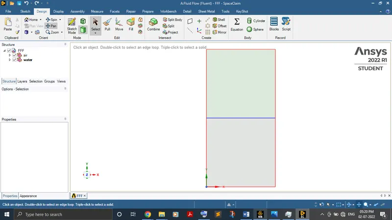
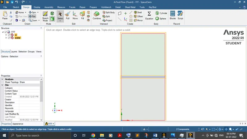
Set the share topology from none to share to share the information between two fluid surface interfaces.

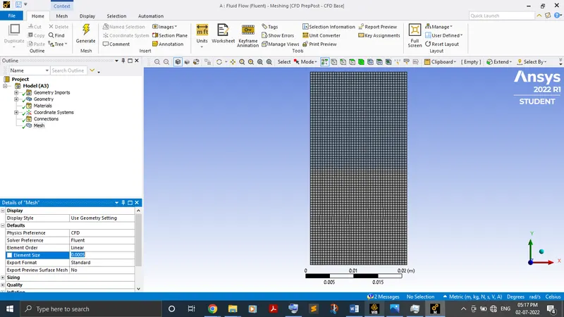
Meshing:

Load the geometry in meshing and mesh it for baseline stuff i.e., element size is 0.5 m.

Setup:

Solver type - Transient state pressure based with gravity in Y as -9.81 m/s

Model

• Laminar viscous model.
• Volume of fluid Multiphase model using implicit scheme for volume fraction parameter.
• Set phase material for each specific phase in specific model.

Material - Fluid (air, water)

Initialize and patch water surface volume of fluid value as 1 and air surface volume of fluid value as 0.

Result:

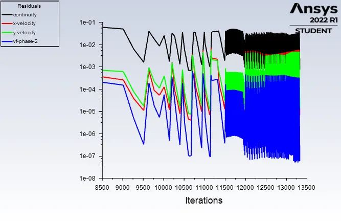
Residual plot:

Animation:

https://drive.google.com/file/d/1wmCexNg_nWBc3rDV70TuLeTFnNalOPsd/view?usp=sharing

Case 2:

Case 2(a): Refining mesh

Except mesh refinement, every step is similar to the previous case.

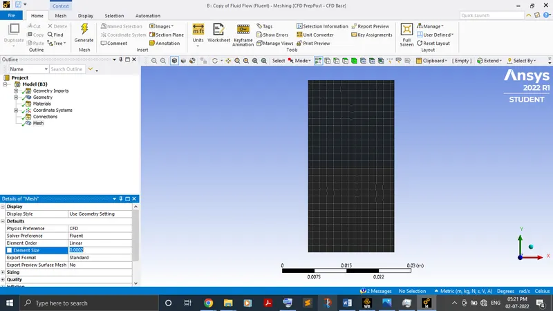
Mesh update: Element size - 0.2m

Result:

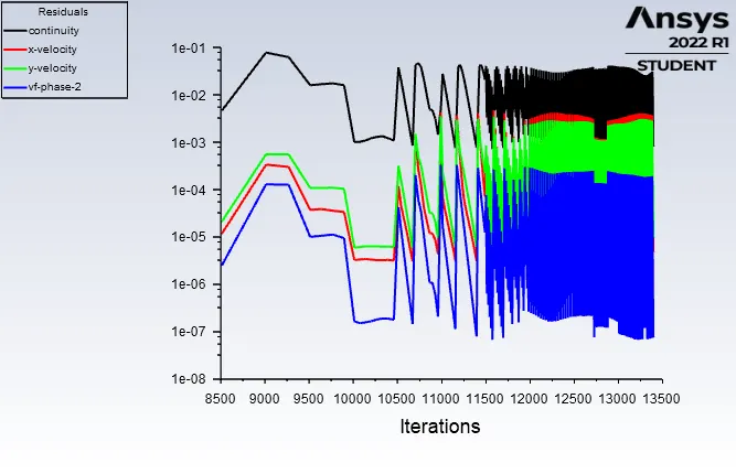
Residual plot:

Animation:

https://drive.google.com/file/d/1mZUry_6wHdLsobUsbsieF42wEfkr7Ynr/view?usp=sharing

Case 2(b): Refined mesh using user defined material

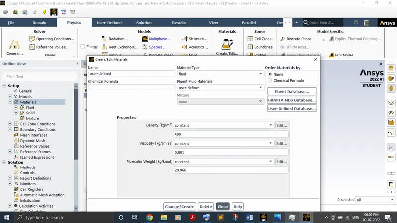
Here, only one change than the previous case is that create the user defined material with the density of 400 kg/m³ and viscosity of 0.001 kg/ ms and use it on the first phase instead of air for the simulation.

Result:

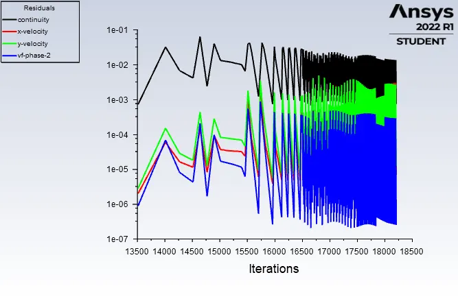
Residual plot:

Animation:

https://drive.google.com/file/d/1WTK4ebzNboGY7wdklG1r8wwP8cOyZsSh/view?usp=sharing

Atwood number:

The Atwood number (A) is a dimensionless number in fluid dynamics used in the study of hydrodynamic instabilities in density stratified flows. It is a dimensionless density ratio defined as

A = (ρ1 - ρ2)/(ρ1+ρ2)

where

ρ1 = density of heavier fluid

ρ2 = density of lighter fluid

Atwood number is an important parameter in the study of Rayleigh–Taylor instability. In Rayleigh–Taylor instability, the penetration distance of heavy fluid bubbles into the light fluid is a function of acceleration time scale.

Atwood number calculation:

Case 1 & 2(a):

ρ1 = 998.2 kg/m³

ρ2 = 1.225 kg/m³

A = 0.996

Case 2(b):

ρ1 = 998.2 kg/m³

ρ2 = 400 kg/m³

A = 0.427

Generally, If Atwood number close to 0, it takes the form of symmetric finger of fluid.

If Atwood number close to 1, the heavier fluid dense through the lighter fluid which forms the large bubbles.

Conclusion:

From the result obtained, we can witness in animation that Atwood number in case 1 & 2(a) are close to 1 which leads to form the large bubbles and heavier fluid (water) quickly dense through the lighter fluid (air). But, in case 2 (b), Atwood number is close to 0.5 which leads to form a small bubbles initially and also heavier fluid (water) takes much more time than the other two cases to dense through the user defined material.

The effect of refining mesh is really helpful to witness the animation result clearly without any patches. The reason why transient state simulation was performed is because to capture & witness each and every small instability variation through animation.