Week 9 - Senstivity Analysis Assignment

Objective:

The aim is to find the sensitivity with respect to the temperature from the GRI mechanism by taking all the reaction and calculates 10 most sensitive reactions.

Theory:

Sensitivity analysis is the study of change of dependent variable with respect to the independent variable.

Sensitivity = ∂y/∂x

In a reaction mechanism, the change of value of parameters is different for different reactions, which means that the parameters are sensitive to some reactions and insensitive (relatively) to some other reactions. There are several reasons for which this happens, as the products and the energy liberated with each reaction are different.

This is done by finding the slope at each time step, for each reaction. Sensitivity value can be negative too, which means that the slope is negative which implies that increase in independent variable and decrease in dependent variable.

Code logic:

• Import and set the necessary libraries and plotting stuffs default.
• The instance object “gas” is created from the solution class.
• Define the reactor object “r” from the Ideal gas reactor class by passing gas object in it.
• Define the reactor network “sim” from the reactor net class by passing the reactor “r” in it.
• Extract and add reactions from the mechanism to sensitivity analysis.
• Set the tolerance for the solution and sensitivity analysis.
• Similarly define the “states” from the solution array class by passing the gas object in it to store the thermodynamic state of it at each time step.
• Within the time loop, “advance” command is used for the purpose of advancing the reaction with time.
• Sensitivity of each reaction is evaluated and store the maximum value of the result.
• Order the reaction and then extract the top 10 results from it.
• Finally, plot the result.

Code:

"""
Constant pressure, adiabatic kinetics simulation with sensitivity analysis
"""

import numpy as np
import matplotlib.pyplot as plt
import cantera as ct
import sys

gas = ct.Solution('gri30.xml')
T = 1500
P = ct.one_atm

gas.TPX = T,P,{'CH4':1, 'O2':2, 'N2':7.52}
r = ct.IdealGasConstPressureReactor(gas, name = 'R1')
sim = ct.ReactorNet([r])
reactions = gas.reaction_equations()

# Extracting and adding reactions from mechanism to sensitivity analysis

n = gas.n_reactions           # Number of reactions in the reaction mechanism
r_nos = (np.linspace(1,n,n))
N = 10

for i in range(n):
	r.add_sensitivity_reaction(i)

# Set the tolerance for the solution and sensitivity analysis

sim.rtol = 1.0e-6   # Relative change in solution should be less than this value
sim.atol = 1.0e-15  # Absolute change in solution should be less than this value

sim.rtol_sensitivity = 1.0e-6   # Relative change in sensitivity should be less than this value 
sim.atol_sensitivity = 1.0e-6  # Absolute change in sensitivity should be less than this value

s_max = [0]*n

states = ct.SolutionArray(gas, extra = ['t'])

for t in np.arange(0, 2e-3, 5e-6):
	sim.advance(t)
	states.append(r.thermo.state, t=1000*t)

	for j in range(n):
		s = sim.sensitivity('temperature',j)

		if abs(s) >= abs(s_max[j]):
			s_max[j] = s

# Ordering the reactions

reactions = [r for s, r in sorted(zip(np.abs(s_max),reactions), reverse=True)]
r_nos = [r for s, r in sorted(zip(np.abs(s_max),r_nos), reverse=True)]
s_max = [s for abs_s, s in sorted(zip(np.abs(s_max),s_max), reverse=True)]

# Extracting top 10 reactions

rplot = reactions[0:N]
r_nos_plot = r_nos[0:N]
splot = s_max[0:N]

# Printing

print("The top %d temperature sensitive reactions are:" % (N))
print("%8s %4s %18s %12s %12s" % ('Reaction Number','|','Reaction','|','Sensitivity'))

for i in range(N):
	print("%11d %8s %26s %4s %10.4f" %(r_nos_plot[i],'|',rplot[i],'|',splot[i]))


# Plotting

fig1, ax1 = plt.subplots()
y_pos = np.arange(len(rplot))
ax1.set_axisbelow(True)
ax1.barh(y_pos, splot, 0.5, align='center', color='black')
ax1.set_yticks(y_pos)
ax1.set_yticklabels(rplot, rotation = 0, fontweight='bold')
ax1.invert_yaxis()
xticks = [-20, -15, -10, -5, 0, 5, 10, 15, 20]
ax1.set_xlabel('Temperature sensitivity')
plt.title('10 most sensitive reactions for the GRI 3.0 mechanism')
plt.tight_layout()
plt.show()

fig2, ax2 = plt.subplots(2,2)
plt.subplot(2,2,1)
plt.plot(states.t,states.T)
plt.xlabel('Time (ms)')
plt.ylabel('Temperature (K)')
plt.subplot(2,2,2)
plt.plot(states.t,states('OH').X)
plt.xlabel('Time (ms)')
plt.ylabel('OH Mole fraction')
plt.subplot(2,2,3)
plt.plot(states.t,states('H').X)
plt.xlabel('Time (ms)')
plt.ylabel('H Mole fraction')
plt.subplot(2,2,4)
plt.plot(states.t,states('CH4').X)
plt.xlabel('Time (ms)')
plt.ylabel('CH4 Mole fraction')
plt.tight_layout()
plt.show()

Result:

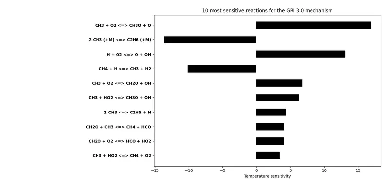
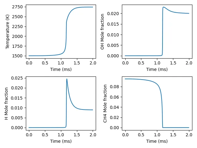
Figure 1: If sensitivity value is positive, which means that the temperature increase the rate of reactions also increase and vice versa if value is negative.

Figure 2: The ignition delay is quiet large when temperature is 1500K. Once, temperature starts to increase, the ignition delay will get reduce. The concentration of each species is varying with respect to time.