Week 3 - Adiabatic Flame Temperature calculation
Adiabatic flame temperature: Final temperature is obtained after the fuel is completely burned
There are 2 types of AFT. They are
- Constant volume
- Constant pressure
When the fuel air mixture takes in constant volume, it increases the internal energy. When the same thing happens in constant pressure, it increases enthalpy.
1. Adiabatic flame temperature variation with Equivalence ratio (In constant volume-chamber):
Equivalent ratio (ɸ): It helps to measure how a mixture is deriving from an ideal stoichiometric reaction.
It is defined as the ratio of the actual fuel/air ratio to the stoichiometric mixture fuel/air ratio.
If ɸ = 1, that is the stoichiometric combustion (both air (O2) and fuel (CO2) is equal)
If ɸ > 1, that is the rich mixture (fuel is more than air)
If ɸ < 1, that is the lean mixture (fuel is less than air)
import matplotlib.pyplot as plt
import cantera as ct
import numpy as np

# Python
# Defining function of enthalpy

def h(T,coeff):
	R = 8.314
	a1 = coeff[0]
	a2 = coeff[1]
	a3 = coeff[2]
	a4 = coeff[3]
	a5 = coeff[4]
	a6 = coeff[5]

	return (a1 + (a2*T/2) + (a3*pow(T,2)/3) + (a4*pow(T,3)/4) + (a5*pow(T,4)/5) + (a6/T))*R*T

# Coefficients for the species from NASA thermodynamic data
# Low temperature

CH4_coeff_l = [5.14987613E+00, -1.36709788E-02, 4.91800599E-05, -4.84743026E-08, 1.66693956E-11, -1.02466476E+04, -4.64130376E+00]
O2_coeff_l = [3.78245636E+00, -2.99673416E-03, 9.84730201E-06, -9.68129509E-09, 3.24372837E-12, -1.06394356E+03, 3.65767573E+00]
N2_coeff_l = [0.03298677E+02, 0.14082404E-02, -0.03963222E-04, 0.05641515E-07, -0.02444854E-10, -0.10208999E+04, 0.03950372E+02]

# High temperature

CO2_coeff_h = [3.85746029E+00, 4.41437026E-03, -2.21481404E-06, 5.23490188E-10, -4.72084164E-14, -4.87591660E+04, 2.27163806E+00]
H2O_coeff_h = [3.03399249E+00, 2.17691804E-03, -1.64072518E-07, -9.70419870E-11, 1.68200992E-14, -3.00042971E+04, 4.96677010E+00]
N2_coeff_h = [0.02926640E+02, 0.14879768E-02, -0.05684760E-05, 0.10097038E-09, -0.06753351E-13, -0.09227977E+04, 0.05980528E+02]
CO_coeff_h = [2.71518561E+00, 2.06252743E-03, -9.98825771E-07, 2.30053008E-10, -2.03647716E-14, -1.41518724E+04, 7.81868772E+00]
O2_coeff_h = [3.28253784E+00, 1.48308754E-03, -7.57966669E-07, 2.09470555E-10, -2.16717794E-14, -1.08845772E+03, 5.45323129E+00]

# Defining function for root solving using Newton Rhapson method
phi = np.linspace(0.1,1.3,50)
def f(T,phi):

	T_std = 298.15
	R = 8.314
	h_CH4_r = h(T_std,CH4_coeff_l)
	h_O2_r = h(T_std,O2_coeff_l)
	h_N2_r = h(T_std,N2_coeff_l)

	H_r = h_CH4_r + (2/phi)*(h_O2_r + (7.52/phi)*h_N2_r)
	N_r = (1 + (2/phi) + (7.52/phi))*R*T_std

	h_CO2_p = h(T,CO2_coeff_h)
	h_H2O_p = h(T,H2O_coeff_h)
	h_N2_p = h(T,N2_coeff_h)
	h_O2_p = h(T,O2_coeff_h)
	h_CO_p = h(T,CO_coeff_h)

	if phi >= 1:
		H_p = (4/phi-3)*h_CO2_p + 2*h_H2O_p + (7.52/phi)*h_N2_p + (4-4/phi)*h_CO_p
		N_p = ((4/phi-3) + 2 + (7.52/phi) + (4-4/phi))*R*T

	elif phi < 1:
		H_p = h_CO2_p + 2*h_H2O_p + (7.52/phi)*h_N2_p + (2/phi-2)*h_O2_p
		N_p = (1 + 2 + (7.52/phi) + (2/phi-2))*R*T

	return (H_p - H_r) - (N_p - N_r)

dT = 1e-6
def fprime(T, phi):
	return (f(T+dT, phi) - f(T,phi))/dT

# Newton Rhapson method

alpha = 0.5
tol = 1e-4
T_guess = 1500
T_aft_py = []

for i in phi:
	while  (abs(f(T_guess,i)) > tol):
		T_guess = T_guess - alpha*(f(T_guess,i)/fprime(T_guess, i))
	T_aft_py.append(T_guess)

# Cantera

gas = ct.Solution('gri30.xml')
T_aft_ct = []

for i in range(0,len(phi)):
	n_tot = 1 + (2/phi[i]) + (7.52/phi[i])
	n_CH4 = 1/n_tot
	n_O2 = (2/phi[i])/n_tot
	n_N2 = (7.52/phi[i])/n_tot
	gas.TPX = 298.15, 101325, {'CH4': n_CH4, 'O2': n_O2, 'N2': n_N2}
	gas.equilibrate('UV','auto')
	T_aft_ct.append(gas.T)

plt.plot(phi,T_aft_py,'o',color='red',label='Python')
plt.plot(phi,T_aft_ct,'o',color='blue',label='Cantera')
plt.xlabel('Equivalent ratio')
plt.ylabel('Adiabatic Flame Temperature')
plt.grid('on')
plt.title('AFT vs Equivalent ratio')
plt.show()
Result:
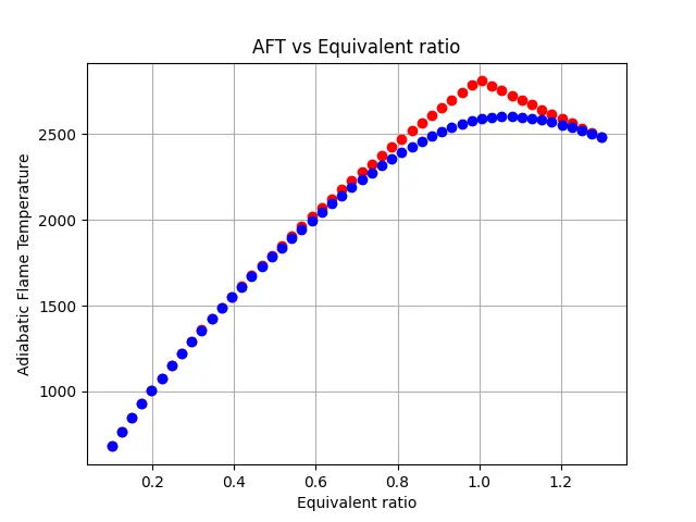
From the result obtained, we can observe that the AFT starts decrease when equivalent ratio goes greater than 1. But a bit variation between using Python & Cantera.
2. Flame temperature variation with Heat loss (In constant pressure-chamber):
Lower heating value (LHV): It helps to determine how much work can be extracted from the fuel.
LHV = (Enthalpy of reactants) – (Enthalpy of products)
import matplotlib.pyplot as plt
import numpy as np

"""
Reaction: CH4 + 2(O2+3.76N2) = CO2 + 2H2O + 7.52N2
"""

# Defining function
def h(T,coeff):
	R = 8.314
	a1 = coeff[0]
	a2 = coeff[1]
	a3 = coeff[2]
	a4 = coeff[3]
	a5 = coeff[4]
	a6 = coeff[5]

	return (a1 + (a2*T/2) + (a3*pow(T,2)/3) + (a4*pow(T,3)/4) + (a5*pow(T,4)/5) + (a6/T))*R*T

# Coefficients for the species from NASA thermodynamic data
# Low temperature

CH4_coeff_l = [5.14987613E+00, -1.36709788E-02, 4.91800599E-05, -4.84743026E-08, 1.66693956E-11, -1.02466476E+04, -4.64130376E+00]
O2_coeff_l = [3.78245636E+00, -2.99673416E-03, 9.84730201E-06, -9.68129509E-09, 3.24372837E-12, -1.06394356E+03, 3.65767573E+00]
N2_coeff_l = [0.03298677E+02, 0.14082404E-02, -0.03963222E-04, 0.05641515E-07, -0.02444854E-10, -0.10208999E+04, 0.03950372E+02]

# High temperature

CO2_coeff_h = [3.85746029E+00, 4.41437026E-03, -2.21481404E-06, 5.23490188E-10, -4.72084164E-14, -4.87591660E+04, 2.27163806E+00]
H2O_coeff_h = [3.03399249E+00, 2.17691804E-03, -1.64072518E-07, -9.70419870E-11, 1.68200992E-14, -3.00042971E+04, 4.96677010E+00]
N2_coeff_h = [0.02926640E+02, 0.14879768E-02, -0.05684760E-05, 0.10097038E-09, -0.06753351E-13, -0.09227977E+04, 0.05980528E+02]
CO_coeff_h = [2.71518561E+00, 2.06252743E-03, -9.98825771E-07, 2.30053008E-10, -2.03647716E-14, -1.41518724E+04, 7.81868772E+00]
O2_coeff_h = [3.28253784E+00, 1.48308754E-03, -7.57966669E-07, 2.09470555E-10, -2.16717794E-14, -1.08845772E+03, 5.45323129E+00]

# Computing the LHV
T_std = 298.15

# Defining function for enthalpy

def f(T,H_loss):

	T_std = 298.15
	R = 8.314
	h_CH4_r = h(T_std,CH4_coeff_l)
	h_O2_r = h(T_std,O2_coeff_l)
	h_N2_r = h(T_std,N2_coeff_l)

	H_r = h_CH4_r + 2*h_O2_r + 7.52*h_N2_r

	h_CO2_p = h(T,CO2_coeff_h)
	h_H2O_p = h(T,H2O_coeff_h)
	h_N2_p = h(T,N2_coeff_h)
	h_O2_p = h(T,O2_coeff_h)
	h_CO_p = h(T,CO_coeff_h)

	H_p = h_CO2_p + 2*h_H2O_p + 7.52*h_N2_p

	LHV = h(T_std,CH4_coeff_l) + 2*h(T_std,O2_coeff_l) - h(T_std,CO2_coeff_h) - 2*h(T_std,H2O_coeff_h)

	return H_p - H_r + (H_loss*LHV)

dT = 1e-4
def fprime(T, H_loss):
	return (f(T+dT, H_loss) - f(T,H_loss))/dT

H_loss = np.linspace(0,1,20)
T_aft = []
H_l = []

for i in H_loss:
	T_guess = 1500.0
	tol = 1e-3
	alpha = 1
	ct = 0


	while ((abs(f(T_guess, i))) > tol):
		T_guess = T_guess - alpha*((f(T_guess, i)/fprime(T_guess, i)))
		ct = ct + 1
	H_l.append(i)
	T_aft.append(T_guess)


plt.plot(H_loss,T_aft)
plt.xlabel('Heat Loss fraction')
plt.ylabel('Flame temperature')
plt.title('Flame temperature vs Heat loss')
plt.show()
Result:
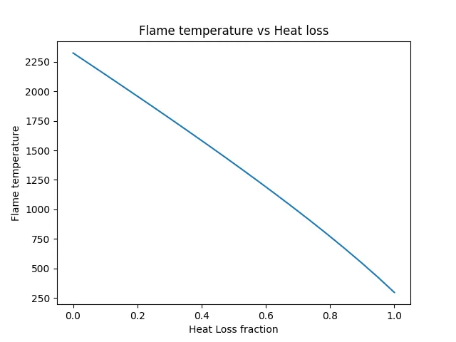
From the result obtained, we can observe that the temperature starts decrease when heat loss increase.
3. Adiabatic flame temperature variation with respect to Alkane, Alkene, Alkyne :
import matplotlib.pyplot as plt

# Defining function of enthalpy
def h(T,coeff):
	R = 8.314
	a1 = coeff[0]
	a2 = coeff[1]
	a3 = coeff[2]
	a4 = coeff[3]
	a5 = coeff[4]
	a6 = coeff[5]

	return (a1 + (a2*T/2) + (a3*pow(T,2)/3) + (a4*pow(T,3)/4) + (a5*pow(T,4)/5) + (a6/T))*R*T

# Coefficients for the species from NASA thermodynamic data
# Low temperature

C2H6_coeff_l = [4.29142492E+00, -5.50154270E-03, 5.99438288E-05, -7.08466285E-08, 2.68685771E-11, -1.15222055E+04, 2.66682316E+00]
C2H4_coeff_l = [3.95920148E+00, -7.57052247E-03, 5.70990292E-05, -6.91588753E-08, 2.69884373E-11, 5.08977593E+03, 4.09733096E+00]
C2H2_coeff_l = [8.08681094E-01, 2.33615629E-02, -3.55171815E-05, 2.80152437E-08, -8.50072974E-12, 2.64289807E+04, 1.39397051E+01]
O2_coeff_l = [3.78245636E+00, -2.99673416E-03, 9.84730201E-06, -9.68129509E-09, 3.24372837E-12, -1.06394356E+03, 3.65767573E+00]
N2_coeff_l = [0.03298677E+02, 0.14082404E-02, -0.03963222E-04, 0.05641515E-07, -0.02444854E-10, -0.10208999E+04, 0.03950372E+02]

# High temperature

H2O_coeff_h = [3.03399249E+00, 2.17691804E-03, -1.64072518E-07, -9.70419870E-11, 1.68200992E-14, -3.00042971E+04, 4.96677010E+00]
N2_coeff_h = [0.02926640E+02, 0.14879768E-02, -0.05684760E-05, 0.10097038E-09, -0.06753351E-13, -0.09227977E+04, 0.05980528E+02]
CO2_coeff_h = [3.85746029E+00, 4.41437026E-03, -2.21481404E-06, 5.23490188E-10, -4.72084164E-14, -4.87591660E+04, 2.27163806E+00]

T_std = 298.15

def f(T,y):

	h_CO2_p = h(T,CO2_coeff_h)
	h_H2O_p = h(T,H2O_coeff_h)
	h_N2_p = h(T,N2_coeff_h)

	h_O2_r = h(T_std,O2_coeff_l)
	h_N2_r = h(T_std,N2_coeff_l)

	x = 2
	if y == 6:
		h_fuel_r = h(T_std,C2H6_coeff_l)
	elif y == 4:
		h_fuel_r = h(T_std,C2H4_coeff_l)
	elif y == 2:
		h_fuel_r = h(T_std,C2H2_coeff_l)


	H_p = (x*h_CO2_p) + (0.5*y) * h_H2O_p + 3.76*(x + (0.25*y)) * h_N2_p
	H_r = h_fuel_r + (x + (0.25*y) * h_O2_r) + (3.76*(x + (0.25*y))*h_N2_r)

	return H_p - H_r

dT = 1e-6
def fprime(T,y):
	return (f(T+dT, y) - f(T,y))/dT

T_g = 1500
tol = 1e-3
alpha = 0.2
ct = 0
y = [6,4,2]
T_aft = []

for i in range(0,len(y)):
	while (abs(f(T_g,y[i]))>tol):
		T_g = T_g - alpha * ((f(T_g,y[i])/fprime(T_g,y[i])))
		ct = ct+1

	T_aft.append(T_g)

plt.bar(['Ethane','Ethene','Ethyne'],T_aft)
plt.xlabel('Hydrocarbon Type')
plt.ylabel('AFT')
plt.title('AFT for different hydrocarbons')
plt.show()
Result:
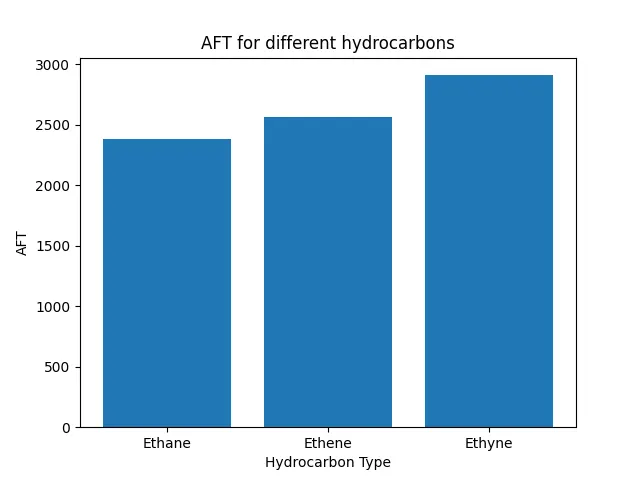
From the result obtained, we can observer that ethyne has more temperature which is due to strong bonding of carbon atoms.
4. Adiabatic flame temperature variation with respect to number of Carbon atom chains :
import matplotlib.pyplot as plt

# Defining function of enthalpy
def h(T,coeff):
	R = 8.314
	a1 = coeff[0]
	a2 = coeff[1]
	a3 = coeff[2]
	a4 = coeff[3]
	a5 = coeff[4]
	a6 = coeff[5]

	return (a1 + (a2*T/2) + (a3*pow(T,2)/3) + (a4*pow(T,3)/4) + (a5*pow(T,4)/5) + (a6/T))*R*T

# Coefficients for the species from NASA thermodynamic data
# Low temperature

CH4_coeff_l = [5.14987613E+00, -1.36709788E-02, 4.91800599E-05, -4.84743026E-08, 1.66693956E-11, -1.02466476E+04, -4.64130376E+00]
C2H6_coeff_l = [4.29142492E+00, -5.50154270E-03, 5.99438288E-05, -7.08466285E-08, 2.68685771E-11, -1.15222055E+04, 2.66682316E+00]
C3H8_coeff_l = [0.93355381E+00, 0.26424579E-01, 0.61059727E-05, -0.21977499E-07, 0.95149253E-11, -0.13958520E+05, 0.19201691E+02]
O2_coeff_l = [3.78245636E+00, -2.99673416E-03, 9.84730201E-06, -9.68129509E-09, 3.24372837E-12, -1.06394356E+03, 3.65767573E+00]
N2_coeff_l = [0.03298677E+02, 0.14082404E-02, -0.03963222E-04, 0.05641515E-07, -0.02444854E-10, -0.10208999E+04, 0.03950372E+02]

# High temperature

H2O_coeff_h = [3.03399249E+00, 2.17691804E-03, -1.64072518E-07, -9.70419870E-11, 1.68200992E-14, -3.00042971E+04]
N2_coeff_h = [0.02926640E+02, 0.14879768E-02, -0.05684760E-05, 0.10097038E-09, -0.06753351E-13, -0.09227977E+04, 0.05980528E+02]
CO2_coeff_h = [3.85746029E+00, 4.41437026E-03, -2.21481404E-06, 5.23490188E-10, -4.72084164E-14, -4.87591660E+04, 2.27163806E+00]

T_std = 298.15

def f(T,x):

	h_CO2_p = h(T,CO2_coeff_h)
	h_H2O_p = h(T,H2O_coeff_h)
	h_N2_p = h(T,N2_coeff_h)

	h_O2_r = h(T_std,O2_coeff_l)
	h_CH4_r = h(T_std,CH4_coeff_l)
	h_C2H6_r = h(T_std,C2H6_coeff_l)
	h_C3H8_r = h(T_std,C3H8_coeff_l)
	h_N2_r = h(T_std,N2_coeff_l)

	if  x == 1:
		y = 4
		h_fuel_r = h(T_std,CH4_coeff_l)
	elif x == 2:
		y = 6
		h_fuel_r = h(T_std,C2H6_coeff_l)
	elif x == 3:
		y = 8
		h_fuel_r = h(T_std,C3H8_coeff_l)


	H_p = (x*h_CO2_p) + (0.5*y) * h_H2O_p + 3.76*(x + (0.25*y)) * h_N2_p
	H_r = h_fuel_r + (x + (0.25*y) * h_O2_r) + (3.76*(x + (0.25*y))*h_N2_r)

	return H_p - H_r

dT = 1e-6
def fprime(T,x):
	return (f(T+dT,x) - f(T,x))/dT

T_g = 1500
tol = 1e-3
alpha = 0.2
ct = 0
x = [1,2,3]
T_aft = []

for i in range(0,len(x)):
	while (abs(f(T_g,x[i]))>tol):
		T_g = T_g - alpha * ((f(T_g,x[i])/fprime(T_g,x[i])))
		ct = ct+1

	T_aft.append(T_g)

plt.bar(['Methane','Ethane','Propane'],T_aft)
plt.xlabel('Hydrocarbon Type')
plt.ylabel('AFT')
plt.title('AFT for different hydrocarbons')
plt.show()
Result:
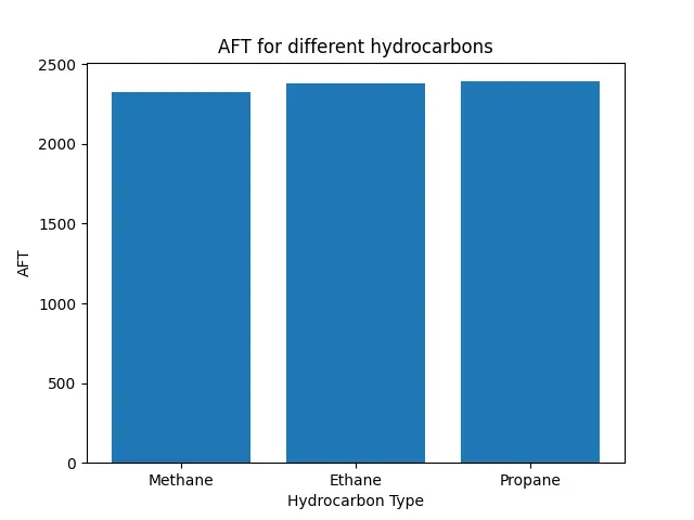
From the result obtained, we can observe that propane has more temperature which is due to strong bonding of carbon atoms.