Week 9 - FVM Literature Review

Finite volume method:

This is a method for representing and evaluating partial differential equations in the form of algebraic equations. In this method, volume integrals in a partial differential equation that contain a divergence term are converted to surface integrals, using the divergence theorem. These terms are then evaluated as fluxes at the surfaces of each finite volume. Because the flux entering a given volume is identical to that leaving the adjacent volume, these methods are conservative. Another advantage of the finite volume method is that it is easily formulated to allow for unstructured meshes. The method is used in many computational fluid dynamics packages. "Finite volume" refers to the small volume surrounding each node point on a mesh.

Finite volume methods can be compared and contrasted with the finite difference methods, which approximate derivatives using nodal values, or finite element methods, which create local approximations of a solution using local data, and construct a global approximation by stitching them together. In contrast a finite volume method evaluates exact expressions for the average value of the solution over some volume, and uses this data to construct approximations of the solution within cells.

Difference between FVM and FDM:

We can’t use FDM on the complex, asymmetrical structure components because FDM only takes the nodal point when it’s linearly aligned to the axis properly. If not so, it takes the nodal point on the next face instead of exact node point. Of course, we can overcome in FDM itself by using variable transformation method which creates new grid(n, є) for a particular space which seems like a normal Cartesian grid(x, y) but results are approximate and takes much time to converge the solution. When compared to FDM, we don’t have any of these complexity in FVM.

Steps to solve 1D linear heat conduction equation:

1. Convert the governing equation into an integral form
2. Apply gauss divergence theorem
3. Choose method to calculate flux terms

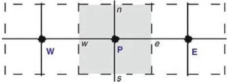
Now, take the governing equation of linear heat conduction equation for 1D with source of the heat generation.

(∂/∂x)*(α*(∂T/∂x)) + S = 0

S – Source

α – Thermal diffusivity

∂T/∂x – Temperature gradient along x axis

Δx – Length of the small control volume along x axis

This equation is applicable throughout inside the volume if the equation at single point is conserved. This could be done by discretization to the whole volume and considering the single point from single volume of discretized.

Now, consider small control volume (dv) and then multiply it to convert into the integral form equation.

∫ ((∂/∂x)*(α*(∂T/∂x)) + S) dv = 0

Now, dv = A*dx

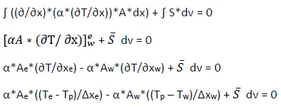
If source term is adding to the cells, then need to have to be done the linearization. We get S_u + S_p*T_p

The above equation is in the format of heat flux in and out with source term. The equation is conserved.

Different types of schemes are used to solve this equation

1. Gradient scheme
2. Interpolation scheme

Gradient scheme:

From the image, we can calculate the temperature gradient in the face (e) which is in between the next node point (E). In order to do this, we use the temperature from the next node point to evaluate the temperature gradient in the face. This scheme is called Gradient scheme.

Interpolation scheme:

We need evaluation of surface and volume integrals in our finite volume formulation, but the surface as well as volume integrals they require the value of the unknown variable at locations other than the computational notes of the CV. So somehow we have to cover with some sort of schemes or mathematical approximation to compute the values at these locations, and that is why we need various types of interpolation formulae.

Types of interpolation in CFD:

1. Upwind interpolation
2. Linear interpolation
3. Quadratic upwind scheme for convective kinematics scheme
4. Hybrid scheme
5. Total variation diminishing scheme
6. Essentially Non-Oscillatory interpolation schemes

Upwind interpolation:

It is essentially used for what we called convection dominated problems, and here the velocity at a given point direction of that velocity that determines the variable values to be used in the interpolation process, the name upwind refers to that we are going to make use of the node which is upwind or upstream of the given node.

Linear interpolation:

Simply, it’s just like a central difference scheme. We have approximate the value of a variable at control volume face centre by linear interpolation of the values at two nearest computational nodes. It is second order accurate. The accuracy is very good but we might have one small problem for advection dominated situations, that this scheme may produce oscillatory solutions, so that is the negative side. On the positive node it is simplest and the most widely used interpolation.

where,

Quadratic upwind scheme for convective kinematics:

It considers the second order derivative term and ignores the third order derivative term. But still it considers as third order accurate. The approximate value of the particular variable at the face centre of the control volume by the quadratic interpolation by using the values at three nearest computational nodes.

where,

Hybrid: It is a blend of CDS and UDS based on the local Peclet number. If the Peclet number is large okay then in that case choose a small values for gamma so that we make use of upwind difference approximation, so this hybrid interpolation scheme it combines the desirable properties of both CDS and UDS.

f_e = νf_CDS + (1-ν)f_UDS

TVD: It is a property of certain discretization schemes used to solve hyperbolic partial differential equations. It the construction of non-oscillatory shock capturing schemes is to require that the total variation of the discrete solution cannot increase. Such schemes are called total variation diminishing (TVD). This criterion has been widely used and also extended to the concept of total variation bounded (TVB) schemes which permit only a bounded increase in the total variation.

f_e = f_p + (0.5*ψ*r*(f_E – f_P))

ψ – flux limiter

Flux limiters:

Most of us might have seen the behaviour of numerical schemes in order to capture shocks and discontinuity that arises in hyperbolic equations. Physically, these equations model the convective fluid flow. It has been observed that low-order schemes are usually stable but quite dissipative in nature around the points of discontinuity/shocks. On the other hand higher-order numerical schemes are unstable in nature and show oscillations in the vicinity of discontinuity. One can have a better understanding of such behaviour by analysing the modified equation of these schemes.

Now as said above one cannot have high order accuracy without oscillations. The objective is to have highly accurate and stable oscillation free schemes. This kind of schemes are known as high resolution schemes. Here we talk only about using flux limiters function to construct high resolution schemes. The idea is to tune the numerical flux of high order and low order scheme using the flux limiter function in such a way that the resulting scheme gives a high order accuracy in the smooth region of flow and sticks with first order of accuracy in the vicinity of shocks/discontinuities.