Week 2 - Flow over a Cylinder.
Objective:
The aim is to simulate the flow over a cylinder and explain the phenomenon of Karman vortex street.
PART-I
- Simulate the flow with the steady and unsteady case and calculate the Strouhal Number for Re= 100.
PART-II
- Calculate the coefficient of drag and lift over a cylinder by setting the Reynolds number to 10,100,1000,10000 & 100000. (Run with steady solver)
- Discuss the effect of Reynolds number on the coefficient of drag.
Potential flow:
In mathematics, potential flow around a circular cylinder is a classical solution for the flow of an inviscid, incompressible fluid around a cylinder that is transverse to the flow. Far from the cylinder, the flow is unidirectional and uniform. The flow has no vorticity and thus the velocity field is irrotational and can be modelled as a potential flow. Unlike a real fluid, this solution indicates a net zero drag on the body, a result known as d'Alembert's paradox.
Kármán vortex street:
In fluid dynamics, a Kármán vortex street (or a von Kármán vortex street) is a repeating pattern of swirling vortices, caused by a process known as vortex shedding, which is responsible for the unsteady separation of flow of a fluid around blunt bodies.
Vortex shedding:
Vortex shedding is an oscillating flow that takes place when a fluid such as air or water flows past a bluff (as opposed to streamlined) body at certain velocities, depending on the size and shape of the body. In this flow, vortices are created at the back of the body and detach periodically from either side of the body forming a Von Kármán vortex street. The fluid flow past the object creates alternating low-pressure vortices on the downstream side of the object. The object will tend to move toward the low-pressure zone.
If the bluff structure is not mounted rigidly and the frequency of vortex shedding matches the resonance frequency of the structure, then the structure can begin to resonate, vibrating with harmonic oscillations driven by the energy of the flow. This vibration is the cause for overhead power line wires humming in the wind and for the fluttering of automobile whip radio antennas at some speeds. Tall chimneys constructed of thin-walled steel tubes can be sufficiently flexible that, in air flow with a speed in the critical range, vortex shedding can drive the chimney into violent oscillations that can damage or destroy the chimney.
Strouhal number:
Strouhal number is a dimensionless number describing oscillating flow mechanisms. The Strouhal number is an integral part of the fundamentals of fluid mechanics.
The Strouhal number is often given as
St = (f*L)/U
where f is the frequency of vortex shedding, L is the characteristic length (for example, hydraulic diameter or the airfoil thickness) and U is the flow velocity. In certain cases, like heaving (plunging) flight, this characteristic length is the amplitude of oscillation. This selection of characteristic length can be used to present a distinction between Strouhal number and reduced frequency:
St = (k*A) / (π*c)
where k is the reduced frequency, and A is amplitude of the heaving oscillation.
Procedure:
Geometry:
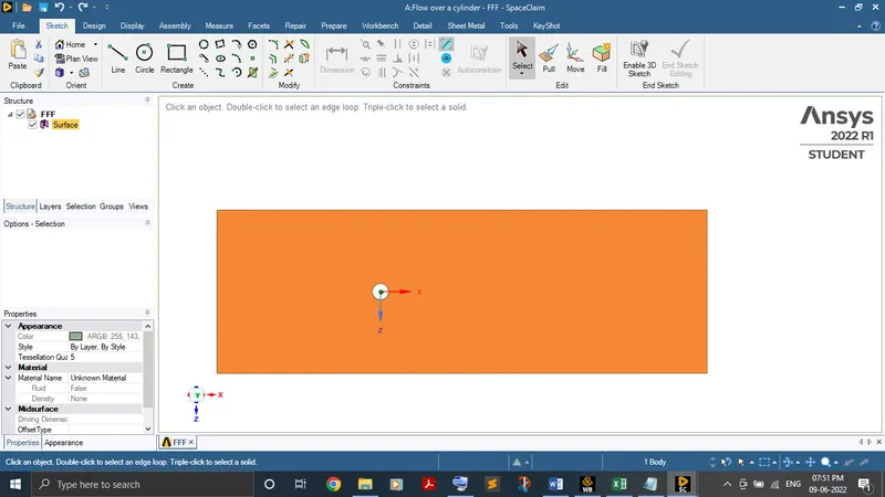
Sketch a rectangle with a dimension of 60 X 20 (in m) and constrain the circle in 20 m length and 10 m height from the left side of the rectangle.
To convert the sketch into the surface, use pull option. Finally, delete the circle surface to get the hole.
Meshing:
Select the edges and create names for it by using named selection.
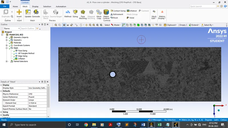
Fix the element size as 0.25 m. Choose the mesh type as triangular.
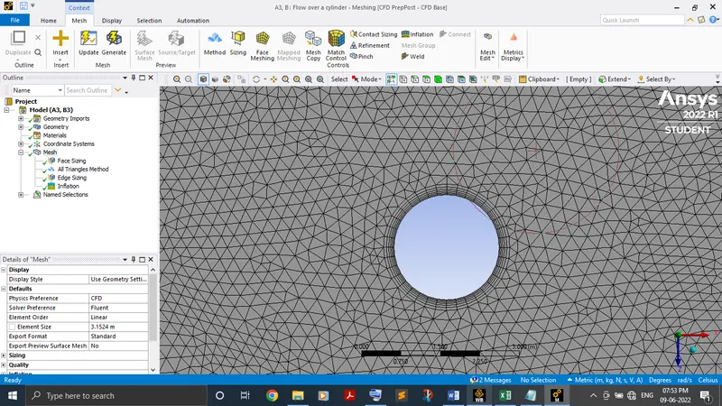
Once we have updated the mesh, if you closely look at the hole it seems to be distorted. So, sizing the circular edge by number of division of 36.
To capture the better result around the wall, create inflation by choosing 1st layer height as 5e-3 m to maximum of 1.2 m gap towards the end layer. Here, we create the maximum layer of 6.
Setup:
Choose solver as steady state.
Choose the laminar from the viscous model.
We need a user defined material to do this simulation. In order to create it, copy the fluid air and rename it.
Boundary conditions are
Velocity inlet – 0.1, 1, 10, 100, 1000 (in m/s) (It’ll according to the Reynolds number).
Pressure outlet – 0 (gauge pressure)
Wall – No slip condition
Reference values:
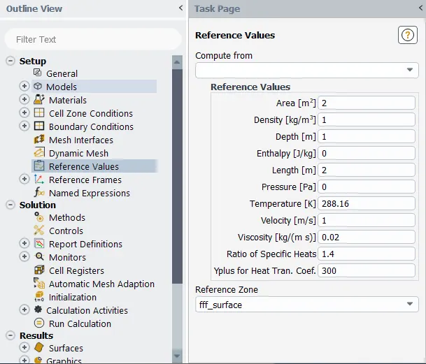
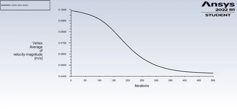
Fix the monitor point in the x axis at the distance of 8 m from the local orgin i.e., from the hole centre.
Results:
Part I:
1. Reynolds number (10):
Velocity = 0.1 m/s
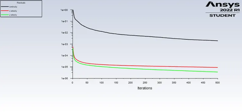
Residual plot:
Monitor point plot:
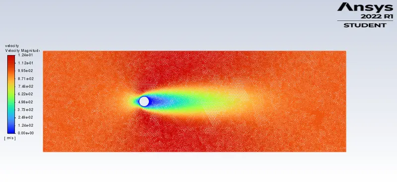
Velocity contour:
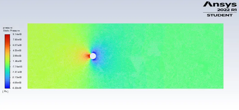
Pressure contour:
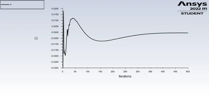
Lift co-efficient:
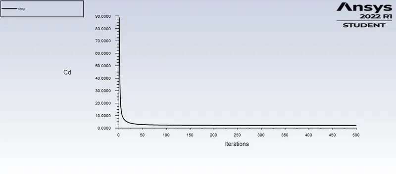
Drag co-efficient:
2. Reynolds number (100 - steady state):
Velocity = 1 m/s
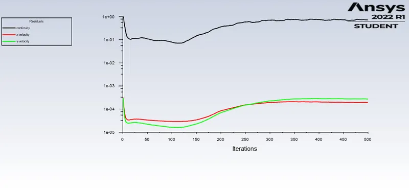
Residual plot:
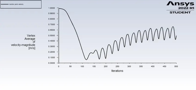
Monitor point plot:
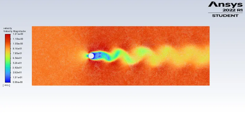
Velocity contour:
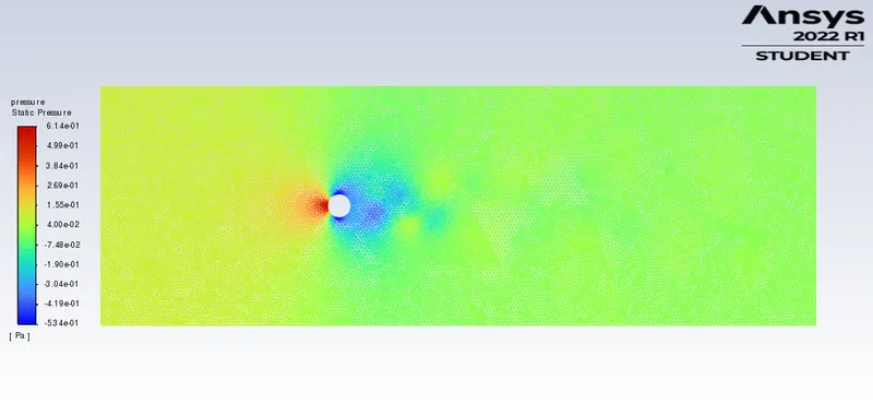
Pressure contour:
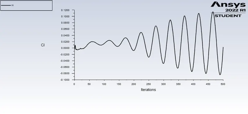
Lift co-efficient:
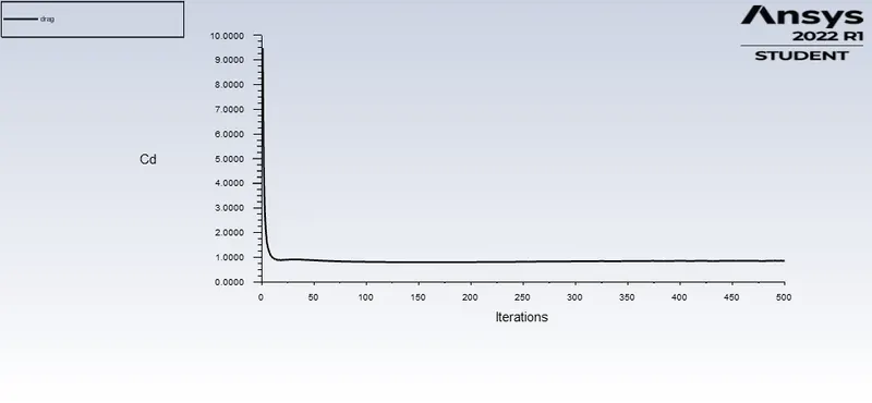
Drag co-efficient:
3. Reynolds number (1000):
Velocity = 10 m/s
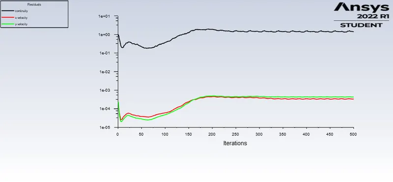
Residual plot:
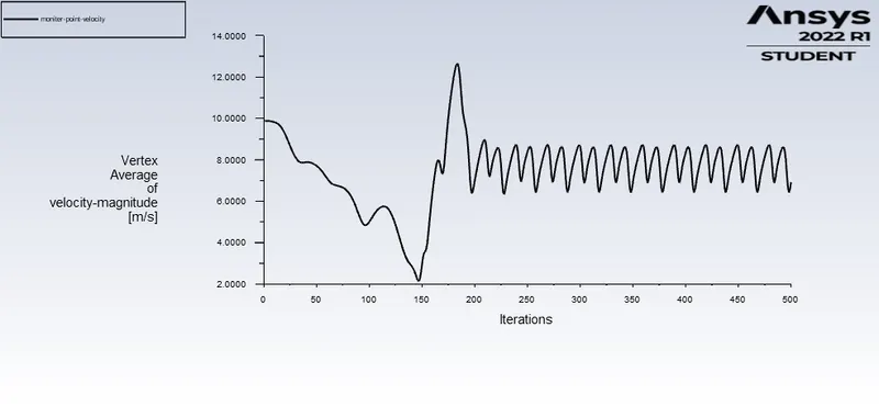
Monitor point plot:
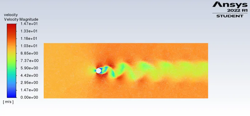
Velocity contour:
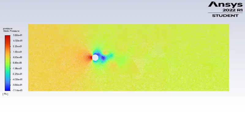
Pressure contour:
Lift co-efficient:
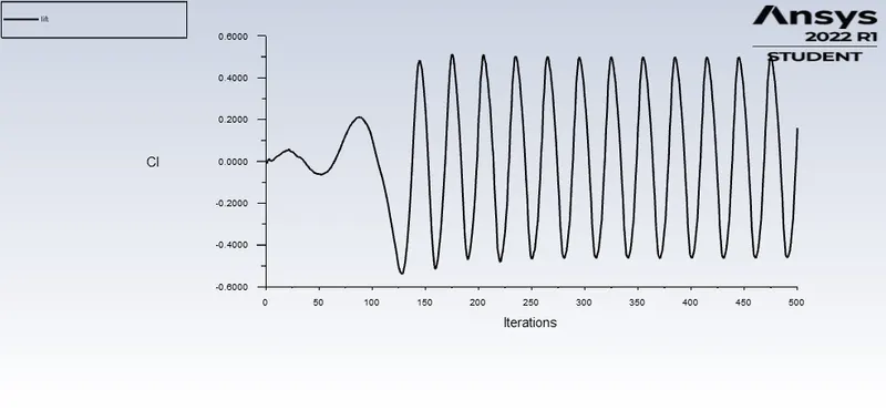
Drag co-efficient:
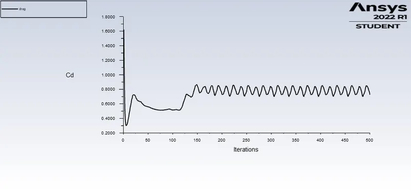
4. Reynolds number (10000):
Velocity = 100 m/s
Residual plot:
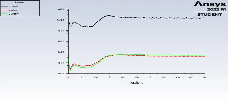
Monitor point plot:
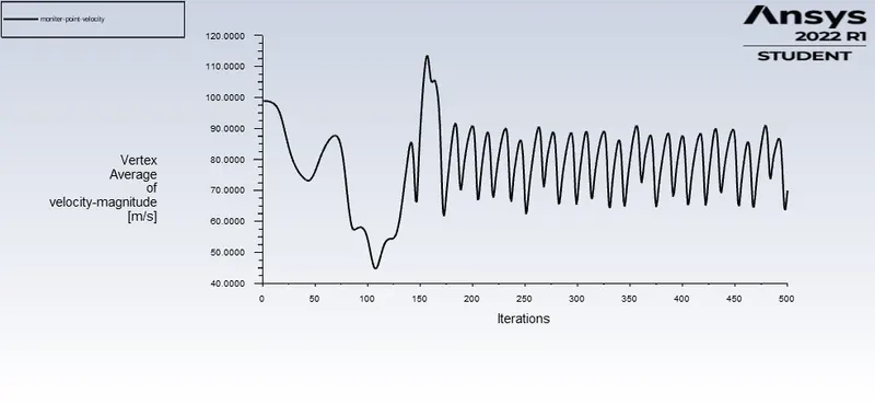
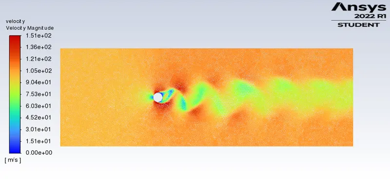
Velocity contour:
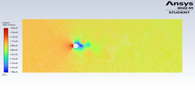
Pressure contour:
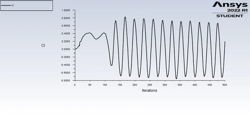
Lift co-efficient:
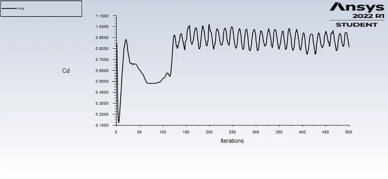
Drag co-efficient:
5. Reynolds number (100000):
Velocity = 1000 m/s
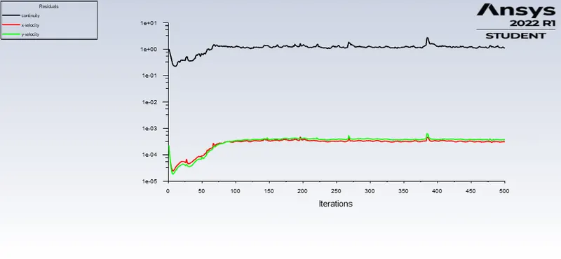
Residual plot:
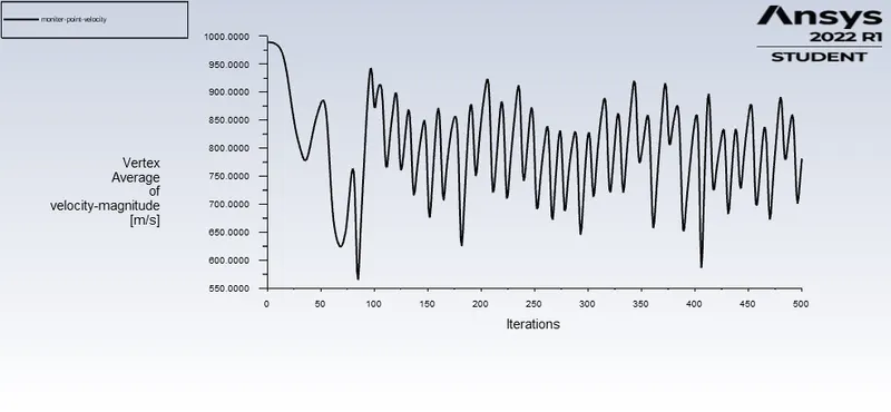
Monitor point plot:
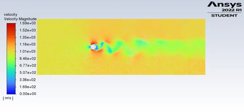
Velocity contour:
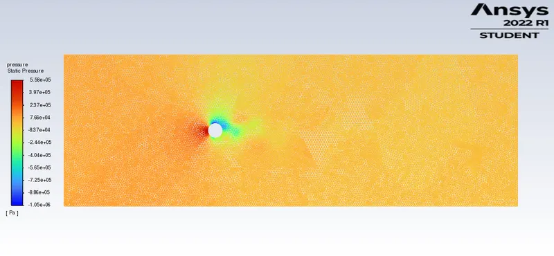
Pressure contour:
Lift co-efficient:
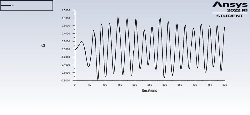
Drag co-efficient:
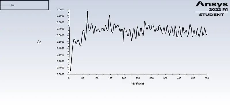
Part II:
1. Reynolds number (100 - unsteady):
Velocity = 1 m/s
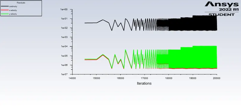
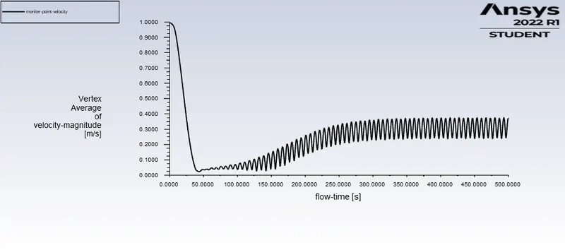
Here, solver setup for this case is transient. Other than that everything is similar as of Part I. Transient simulation gives the result for each and every time step. But steady state simulation gives result only for the final step. Best part of using the transient is even for Re = 40, we can witness the flow seperation.
Residual plot:
Monitor point plot:
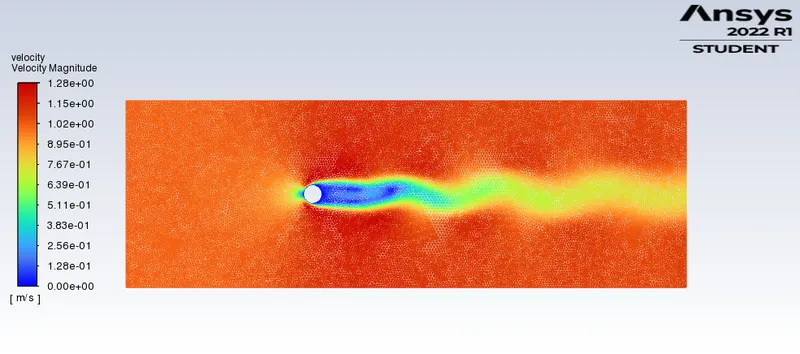
Velocity contour:
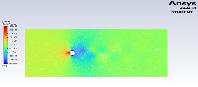
Pressure contour:
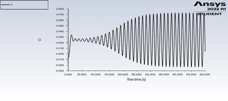
Lift co-efficient:
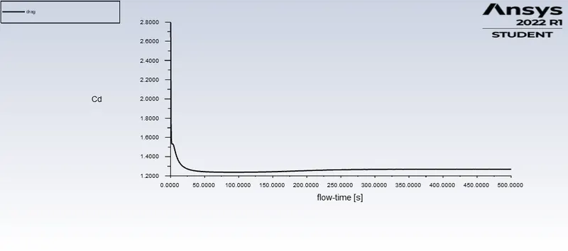
Drag co-efficient:
Strouhal number:
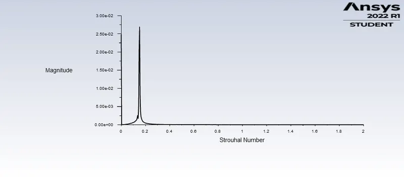
To find the Strouhal number using ansys fluent, go to the results and expand plot and choose FFT (Fast Fourier Transform).
Fourier transform is mainly done to convert a sequence of signals in the time domain to its frequency.
In FFT, set x-axis as strouhal number and y-axis as magnitude. Load data file from the previously completed simulation and plot the result. Finally, write FFT to file and click on write FFT.
Here, Strouhal number is 0.152 for the unsteady simulation.
Conclusion:
From the result obtain, we can say that where the flow strikes the wall of the cylinder at 0 degree angle, there is no velocity and that point is called stagnation point. So, the pressure is high at this point. When the fluid flows over the cylinder, it forms the wake region which means that the region of recirculating flow immediately behind a moving or stationary blunt body, caused by viscosity, which may be accompanied by flow separation and turbulence. In this region, pressure is low due to high velocity. Also, when the Reynolds number increases drag coefficient decreases due to velocity increases in our case.
References:
https://www.sciencedirect.com/science/article/pii/S0307904X08000243
https://en.wikipedia.org/wiki/Strouhal_number
https://en.wikipedia.org/wiki/Potential_flow_around_a_circular_cylinder
https://skill-lync.com/knowledgebase/how-to-perform-a-fft-using-ansys-fluent
https://en.wikipedia.org/wiki/K%C3%A1rm%C3%A1n_vortex_street