Calculating the Stretch Ratio by comparing the ELFORM (-2,-1,1,2) with Ogden_Material Model in LS-DYNA
Aim:
1) To Create a block of 10mmx10mmx10mm dimension with 10 elements for each direction and use the material card attached (Ogden_Material.k).
2) Use appropriate boundary conditions to simulate uniaxial tensile behavior for the model.
3) Compare the results of the simulation with ELFORM = 1, 2, -1, -2 by plotting Engineering Stress vs Stretch Ratio up to stretch ratio 5.
4) To use a proper solver (Implicit/Explicit).
Theory:
An Ogden model is a hyperelastic material model that can be used for predicting the nonlinear stress-strain behavior of materials such as rubber or polymer. Ogden's model was introduced Ogden in 1972. The Ogden model has been frequently used for the analysis of rubber components like O-ring and seal. Even though the Ogden model is a hyperelastic material model, its strain energy density function is expressed by the principal stretch ratio.
Procedure:
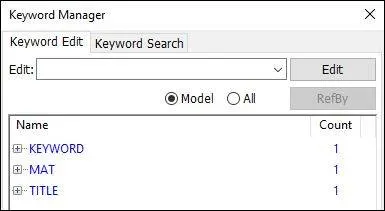
1) The given LS-Dyna keyword file is opened in LS-PrePost using the option File->Open->LS-Dyna Keyword File. The imported keyword file consists of only the Ogden material card as shown in the image given below.
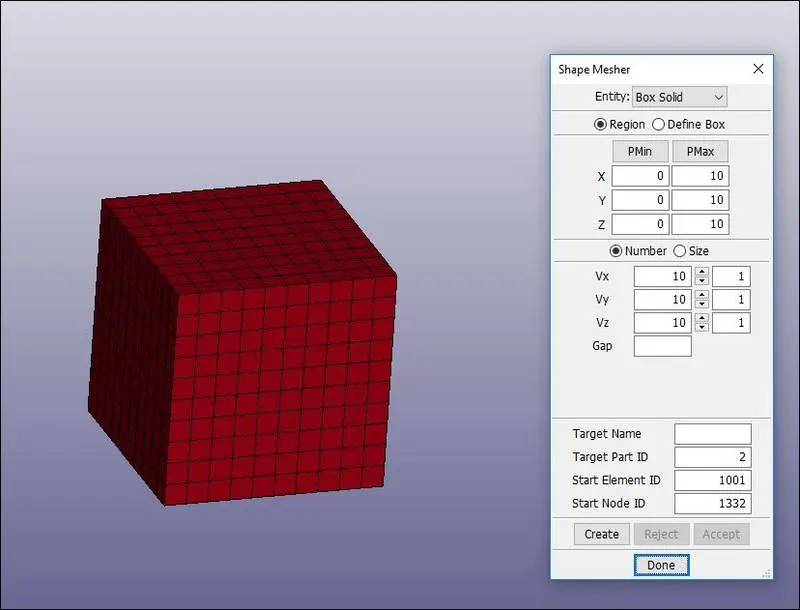
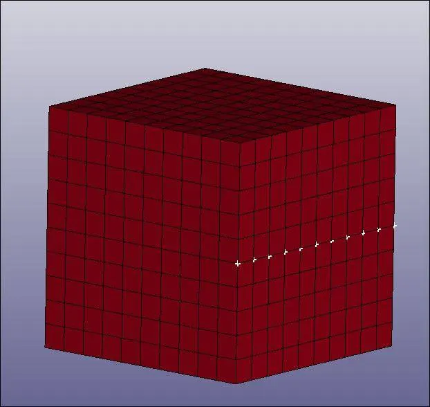
2) The FE model of a solid block of 10mmx10mmx10mm dimension with 10 elements for each direction is created using the Shape Mesher under the mesh tab as shown in the image given below.
Section Creation:
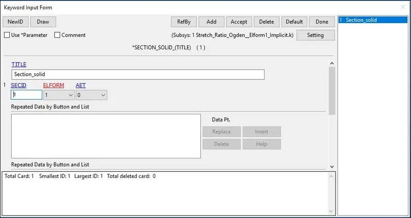
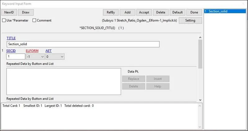
3) The section properties of the FE model created is assigned as a solid element with different ELFORM such as,
Case (1). ELFORM = 1, constant stress solid element.
Case (2). ELFORM = -1, Fully integrated S/R solid intended for elements with poor aspect ratio, efficient formulation.
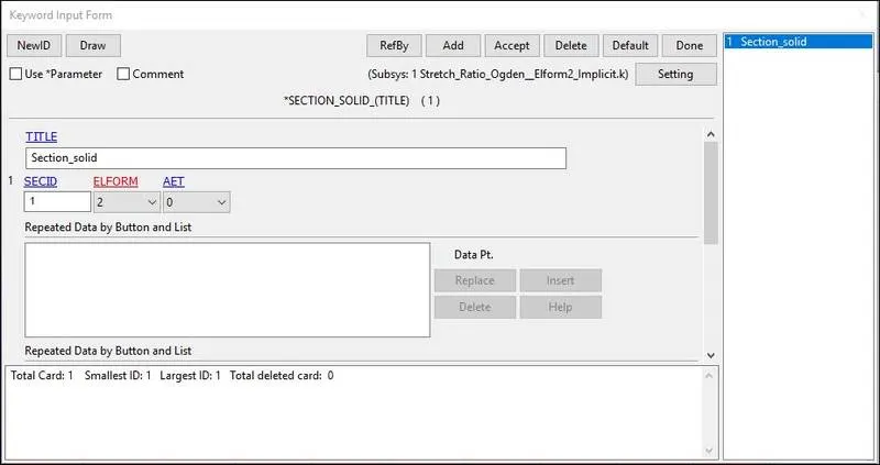
Case (3). ELFORM = 2, Fully integrated S/R solid
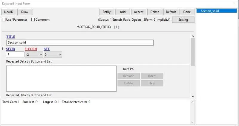
Case (4). ELFORM = -2, Fully integrated S/R solid intended for elements with poor aspect ratio, accurate formulation.
The section definition for each case is shown in the images given below.
Material:
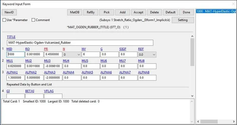
4) The material card given in the below image is already provided in the keyword file, the unit system followed is gm-mm-ms and it is assigned to the solid block part.
Assigning Material and Section to Part:
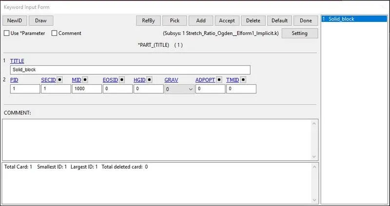
5) The material and section properties are assigned to the solid part as shown in the image given below.
Boundary Conditions:
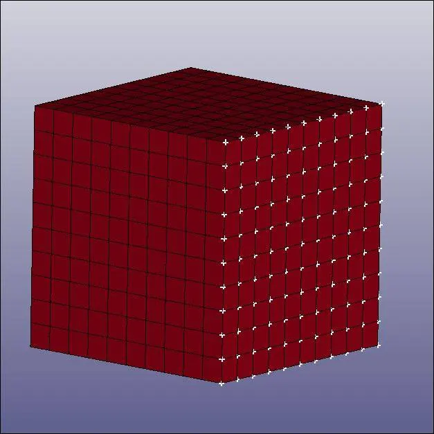
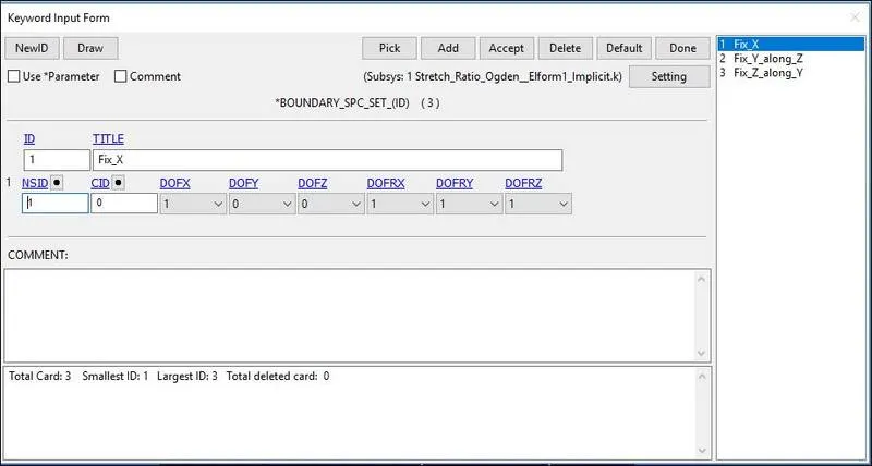
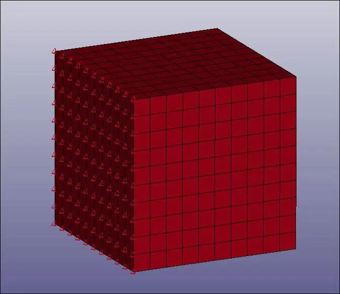
6) To perform the uniaxial tensile test on the specimen, the nodes of one of the faces are fixed along the X-axis.
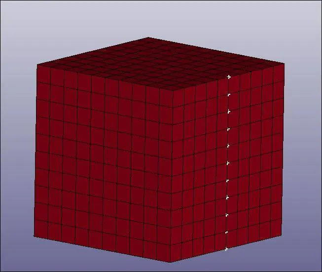
7) Then we fix the vertical middle nodes along Z- direction fixed in Y-direction.
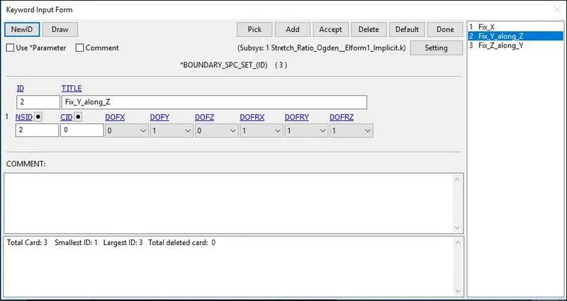
8) Then we fix the horizontal Middle nodes along Y-direction fixed in Z-direction.
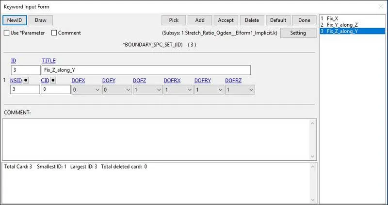
9) The Nodes in the moving face are selected for applying load.
10) The minimum load to be applied on the moving surface to attain a stretch ratio of 5, is calculated by using the following relation,
Engineering strain, `ε_e=(δl)/l`
Stretch ratio, `λ=1+ε_e`
`5=1+(δl)/10`
`δl=40mm,`
Hence, the minimum value of 50mm is taken to define the load curve.
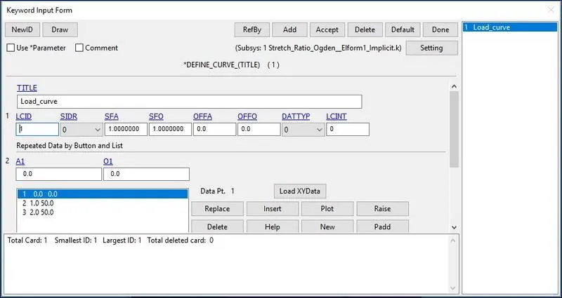
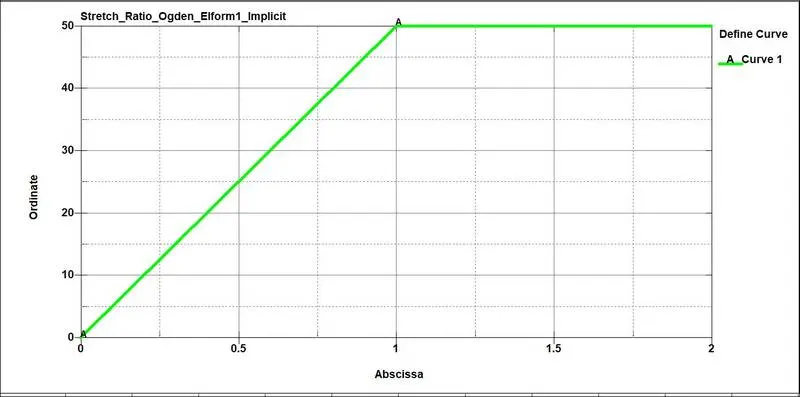
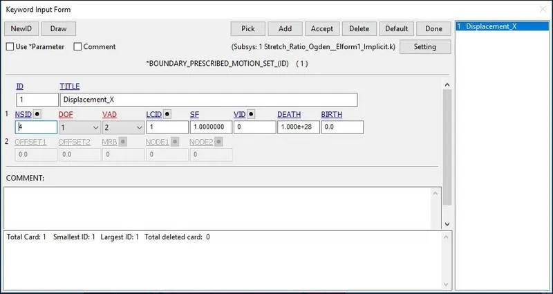
11) The node-set and load curve ID's are assigned to the prescribed motion set so the selected nodes move along the X-direction.
Control Cards:
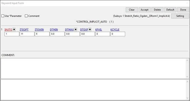
12) CONTROL_IMPLICIT_AUTO card as shown in the below image is used for automatic time step control during implicit analysis. Input value for Automatic time step control flag = IAUTO = 1.
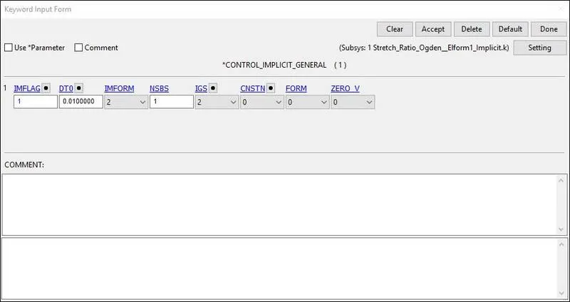
13) CONTROL_IMPLICIT_GENERAL card as shown in the below image is used to activate implicit analysis and define associated control parameters. This keyword is required for all implicit analyses.
The input value for IMFLAG=Implicit/Explicit switching flag = 1 (implicit analysis)
DT0=Initial time step size for implicit analysis = 0.01.
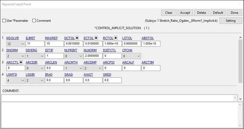
14) CONTROL_IMPLICIT_SOLUTION card as shown in the below image is used to specify whether a linear or nonlinear solution is desired. The default values are set as it is in the card.
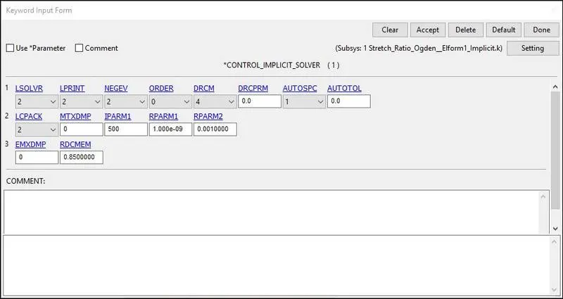
15) CONTROL_IMPLICIT_SOLVER card as shown in the below image is used for implicit calculation.
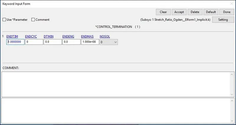
16) The control termination function as shown in the below image is enabled to specify the end time of the simulation. The termination time is set for 1 ms.
Database:
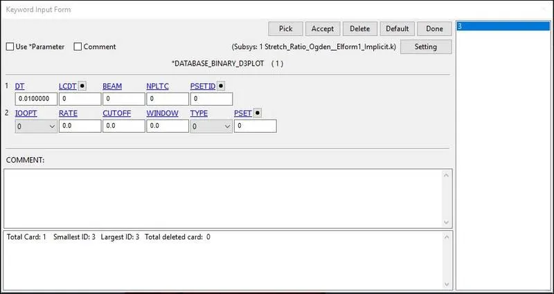
17) The time step value of 0.01 ms is given for the BINARY_D3PLOT as shown in the below image and the DATABASE_ASCII option for GLSAT and ELOUT.
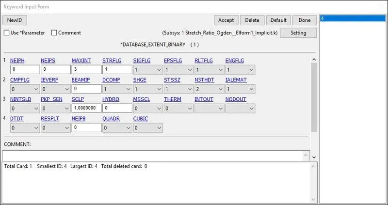
18) The DATABASE_EXTENT_BINARY card with STRFLG =1, as shown in the below image is used to compute the elastic strain in the model.
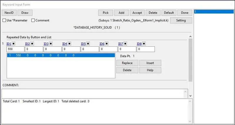
19) The DATABASE_HISTORY_SOLID card as shown in the below image is used to compute the stress/strain of a 550 node in the model.
Model Check:
20) The keyword file created is checked for errors using the option keyword manager>model check as shown in the below image.
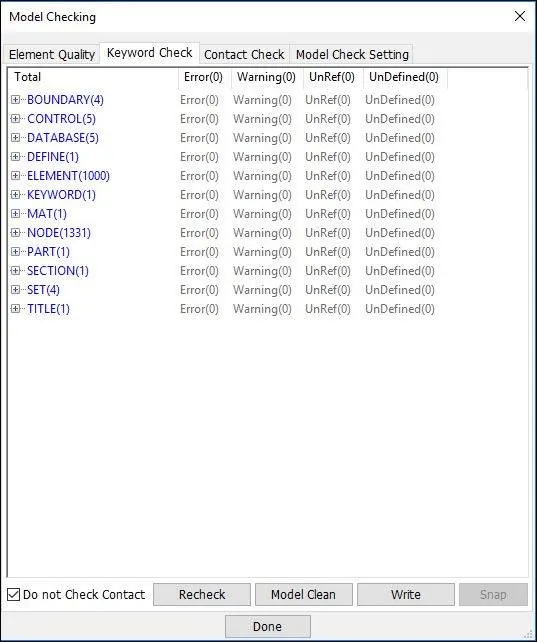
21) The keyword file is saved using the ‘.k’ extension and is made to run in the solver by getting normal termination messages for different cases of ELFORM.
Results and Discussion:
Animation Contours:
The D3plot output file is opened in LS-PrePost using the option File->open->LS-Dyna binary plot.
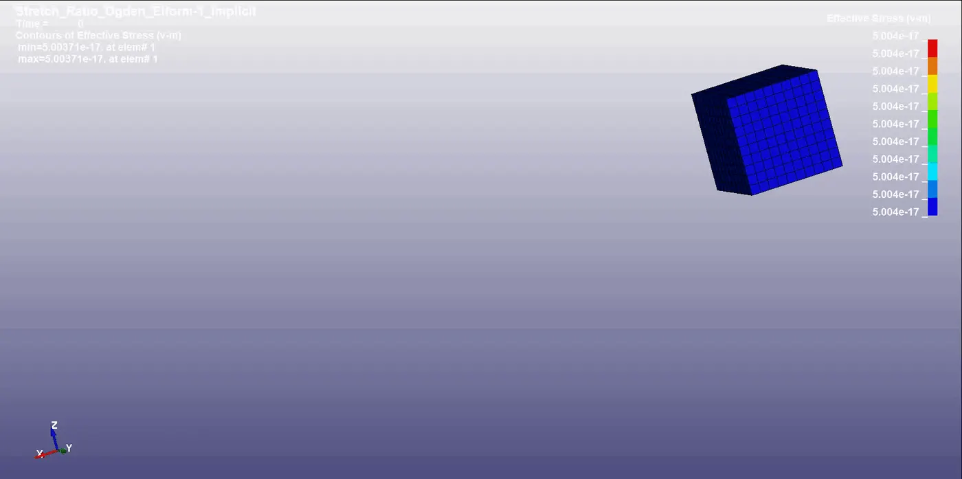
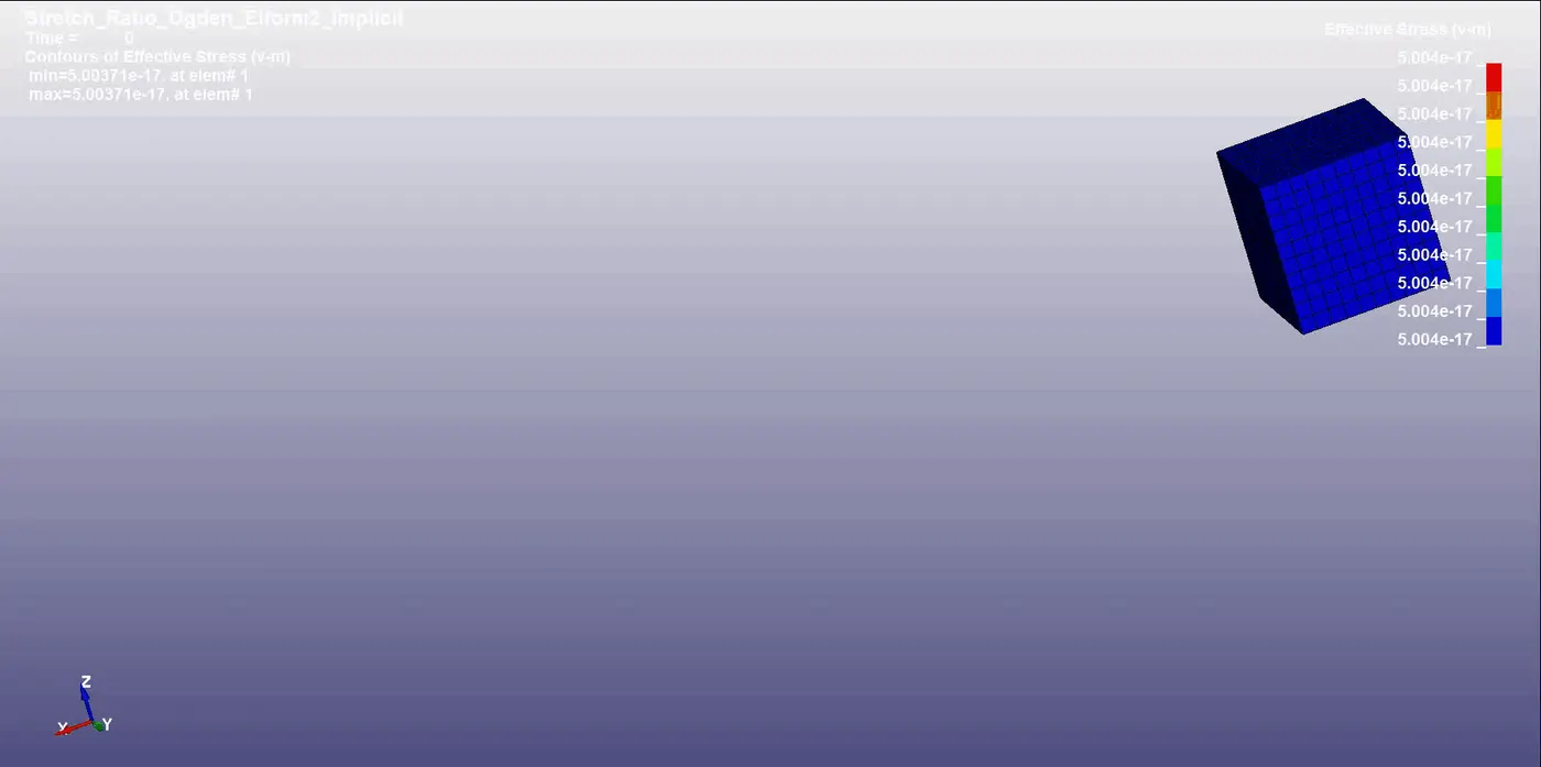
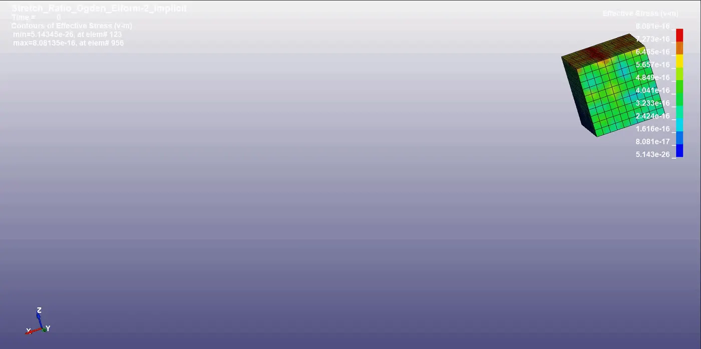
2) We first get the animation contours for von mises data for all the cases.
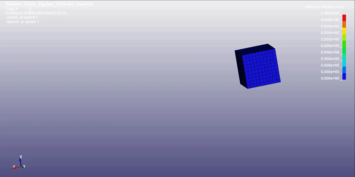
3) then we also get the animation contours for X-axis strain data for all the cases.
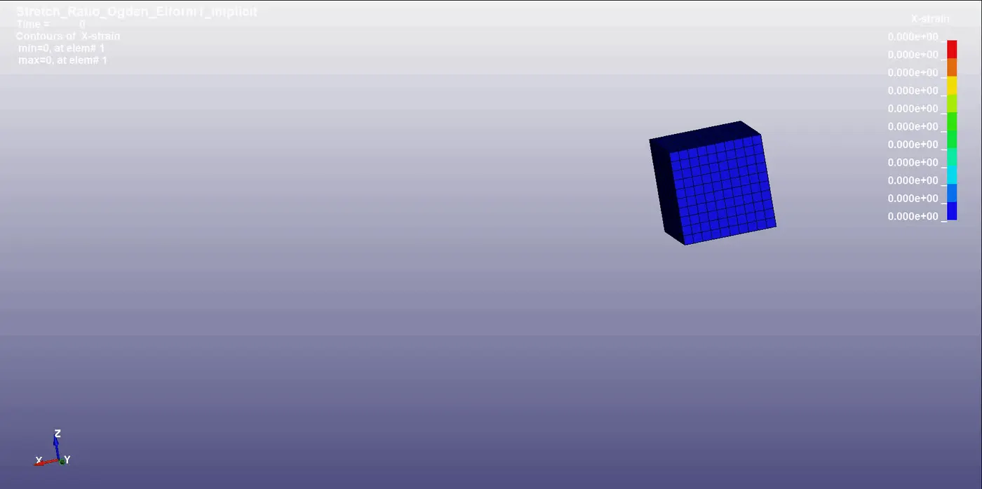
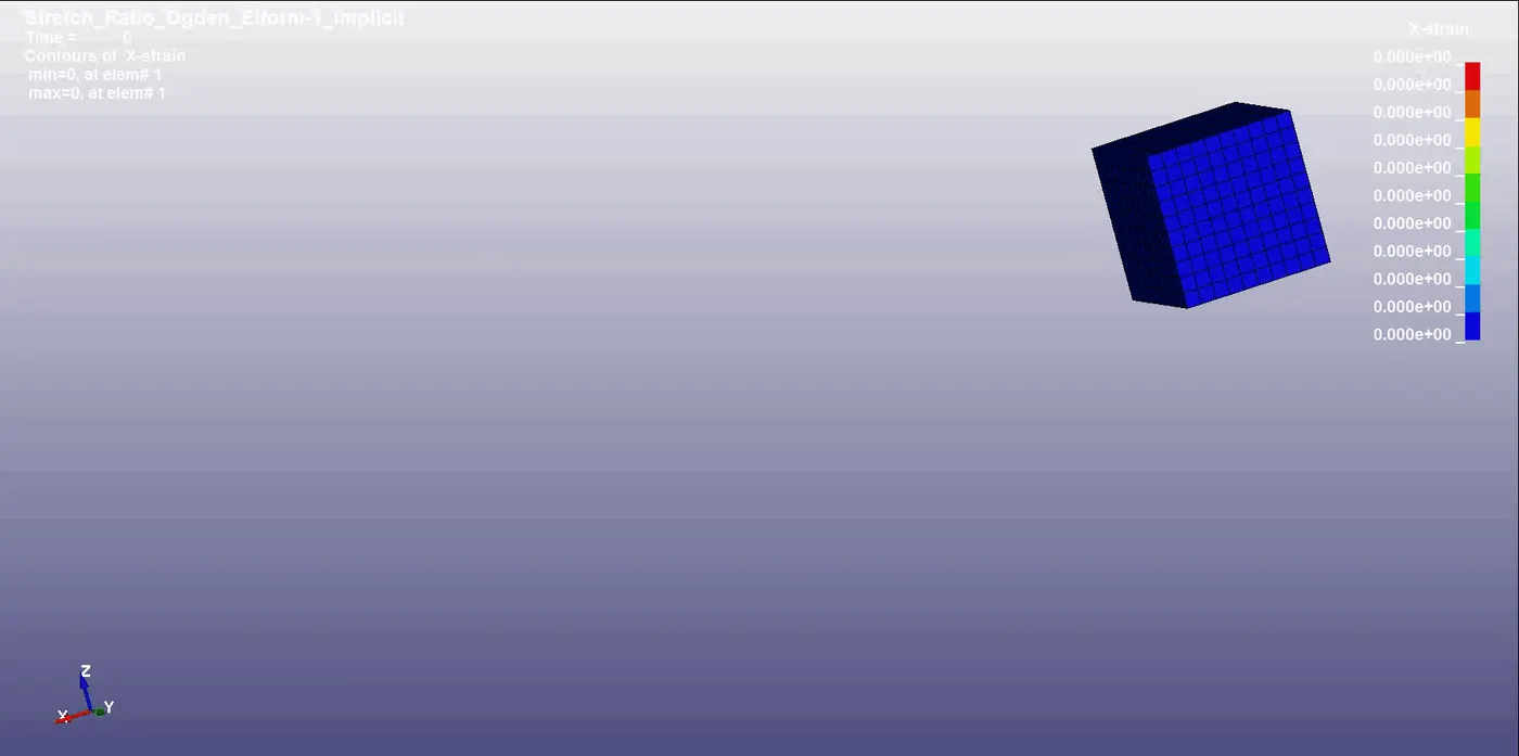
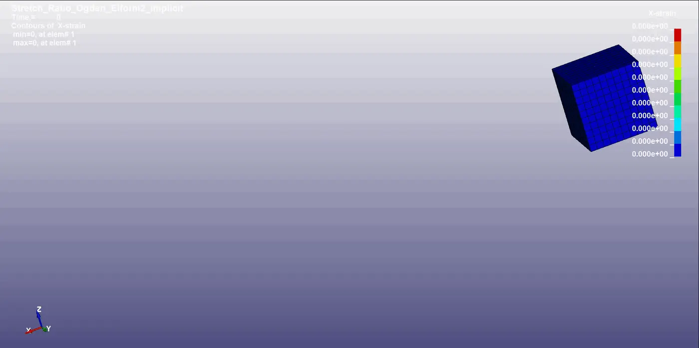
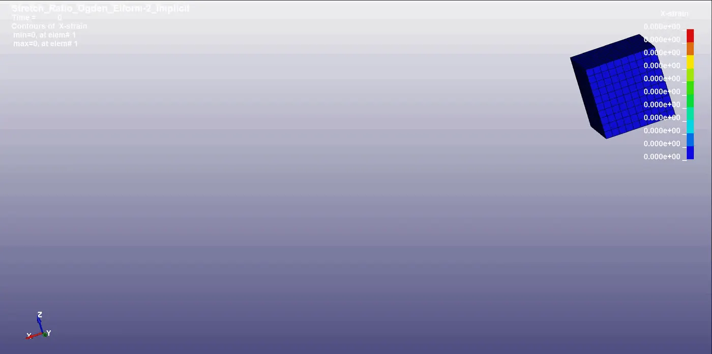
4) From the above contour animations we observe that the maximum value of von mises stress for case 1, 2, 3, and 4 are 5.025 MPa, 5.0239 MPa, 5.0312 MPa, 5.0239 MPa respectively. The maximum value of X-strain for cases 1, 2, 3, and 4 are 1.7885, 1.7878, 1.789, 1.7879 respectively. There is a small variation in the stress value but the strain value is almost the same for different cases.
Calculation of Engineering stress/strain and stretch ratio:
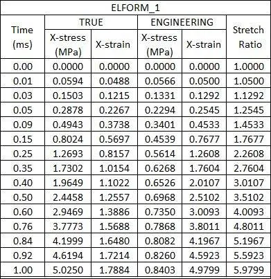
5) In LS-DYNA always the output of stress and strains which we get from the Post Fringe Comp Stress/Strain are given as true stress and strains. To find the engineering stress/strain and stretch ratio following relations are used,
We know that, True stress, `σ_t=σ_e (1+ϵ_e )`
Engineering stress, `σ_e=σ_t/((1+ϵ_e ) )`
Similarly, True strain, `ϵ_t=ln(1+ϵ_e)`
Engineering strain, `ϵ_e=e^(ϵ_t )-1`
Stretch ratio, `λ=1+ε_e`
6) We use excel to calculate our Engineering Stress (`ϵ_e`) and Stretch Ratio (`λ`) using the above relations. The images of the excel tables for all the cases are given below.
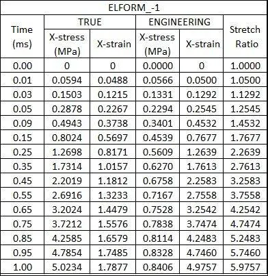
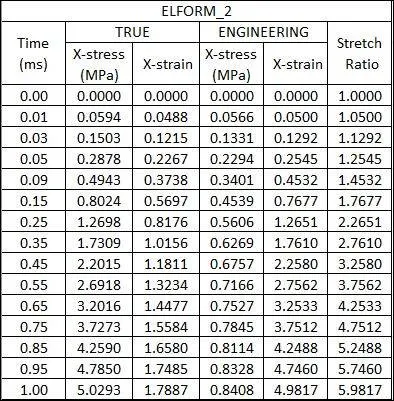
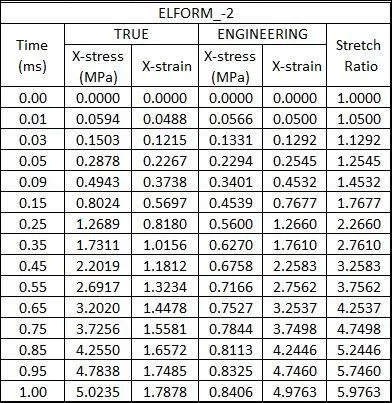
7) We also plot the Engineering Stress (`ϵ_e`) vs Stretch Ratio (`λ`) graph for all the cases as shown in the images given below.
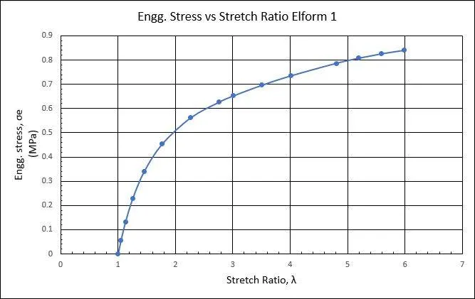
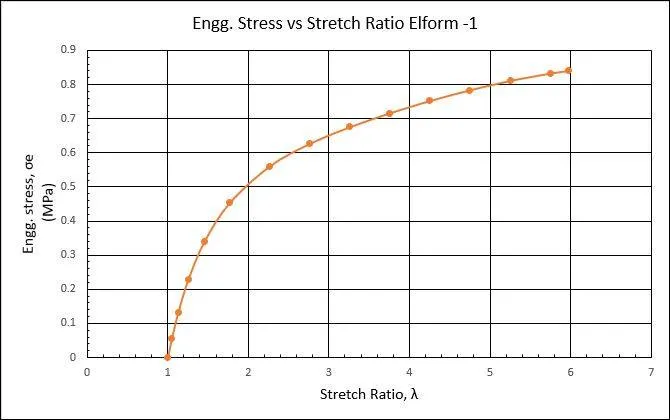
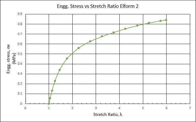
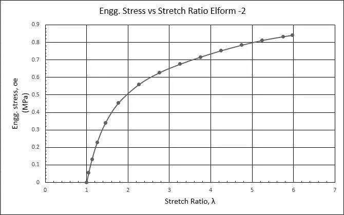
8) From the graphs plotted for Engg. Stress vs Stretch Ratio for different cases, the Engg. stress value corresponding to a stretch ratio of 5 is 0.8 MPa approximately. The output from different cases of elform gives approximately the same results since the model and loading conditions are simple.
9) In the actual Nominal Stress vs Stretch Ratio plot for Ogden material the value of nominal stress for a stretch value of 5 is approximately 1.8 MPa but from the simulation result, the value of stress is 0.8 MPa. It is observed that a variation of 1 MPa is caused in the simulation for the uniaxial tension test for Ogden material because of the non-linearity of the material and the relatable boundary condition applied for the model.
Conclusion:
1) A FE model of solid block was created with Ogden material to simulate an uniaxial tension test for different cases of ELFORM (1, -1, 2, -2).
2) The Engineering stress/strain and stretch ratio was calculated to plot a graph of Engg. stress vs stretch ratio up to stretch ratio 5.
3) The Engineering stress value for a stretch value 5 from the simulation for different ELFORM was approximately equal to 0.8 MPa, but from the actual graph, it was equal to 1.8 MPa with a difference of 1 MPa.
4) The uniaxial tension test was solved using an implicit solver since the analysis is similar to a quasi-static analysis on a hyperelastic non-linear material with slow steady loading conditions.