Analysis and Comparison of different Material Laws with a Sphere and Rupture Plate Model in Radioss
Aim:
1) To run the seven cases as mentioned in the below image.
The seventh case is running the model with LAW 36.
2) Plotting all the necessary contour and 2D plots energy plots for all the cases.
3) Tabulating the results obtained from simulating each case.
4) Comparing the results with each other and finally stating which of these cases would represent the on-field scenario.
Procedure:
1. Case-1:
1) In case 1, we run the simulation with recommended properties, default material parameters and default failure properties.
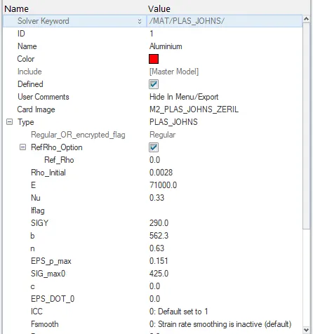
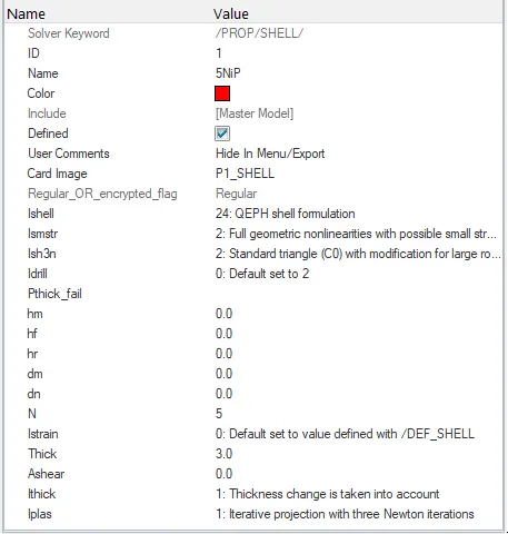
2) We first import the rad file 'FAILURE_JOHNSON_0000.rad' and we run the simulation with default material and shell properties as shown in the images given below.
3) We run the simulation by going to the analysis module and clicking on radioss option with the starter file name as 'Law2_epsmax_failure_0000.rad' as shown in the image given below.

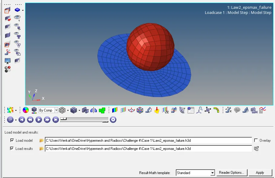
4) We go to Hyperview and import the file 'Law2_epsmax_failure.h3d' then, then we check for contour plot on Von mises stress with simple average method as shown in the image given below.
5) After running the von mises animation we see that the elements in the plate after a point get deleted as shown in the animation given below.
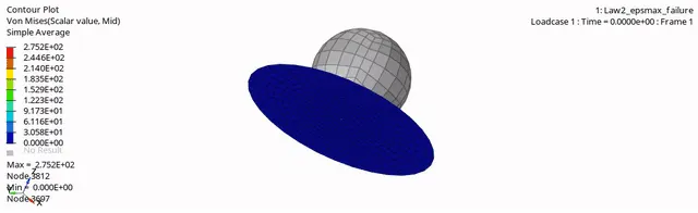
The max von mises stress was found out to be 275.2 MPa.
6) We look out for the energy error and mass error in 'Law2_epsmax_failure_0001.out' in the form of the text editor as shown in the image given below.
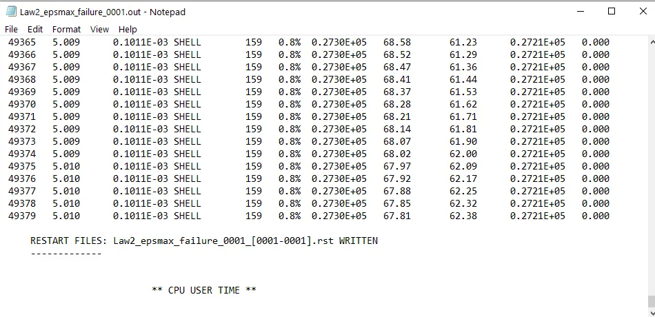
Energy Error: 0.8%
Mass Error: 0
Elapsed Time: 138.33 secs
No of Cycles: 49380
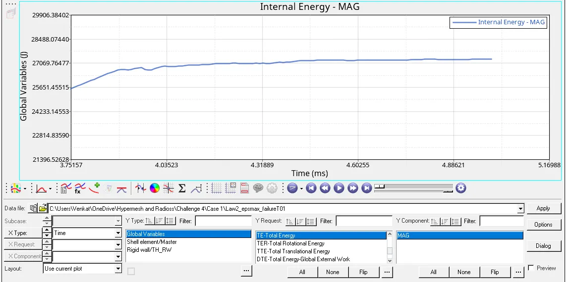
7) We then, proceed to plot the graphs the results with the help of Hypergraph 2D. We plot graphs for all the energies which include internal energy, kinetic energy and total energy. We don't plot graph for hourglass energy since we are using recommended shell formulation properties. The plots are shown in the images given below.
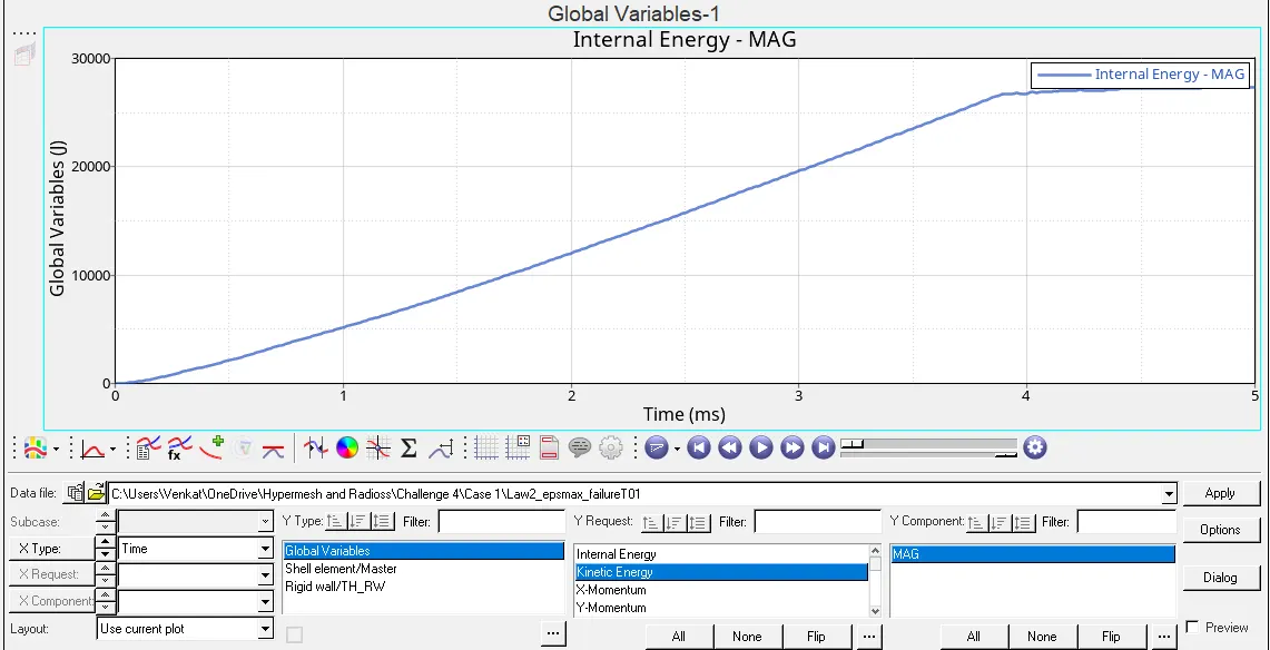
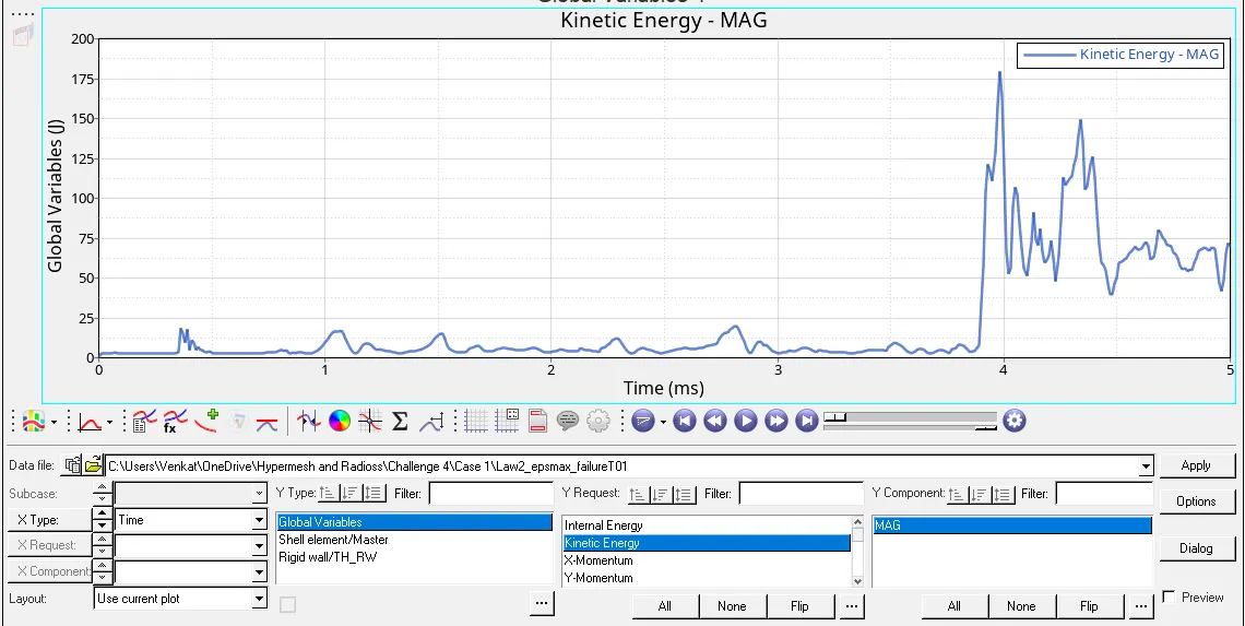
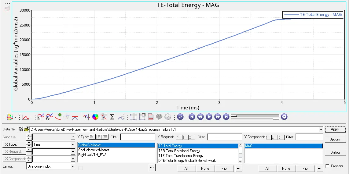
8) We see that in the internal energy plot the oscillating region in the below image is called the Strain Hardening Process. Beyond this region due to High Elongation loads it will undergo plastic strain followed by severe plastic strain and finally fails.
2. Case-2:
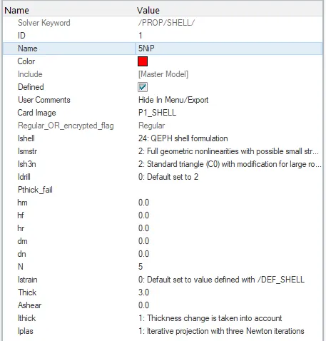
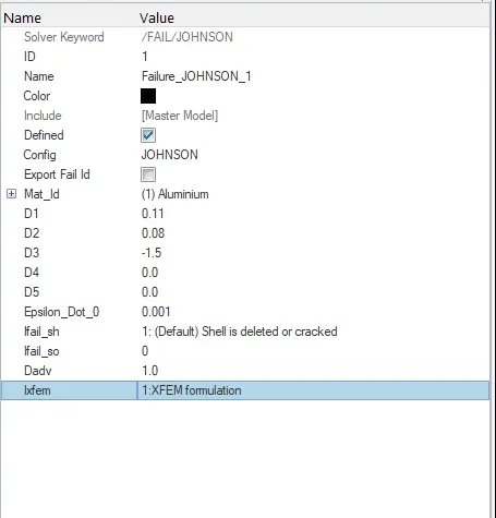
1) In case 2, we run the simulation with recommended properties, default material parameters and we change the values of Ifail_sh=1, Dadv= 1 & Ixfem= 1 in the failure card.
2) We first import the rad file 'FAILURE_JOHNSON_0000.rad' and we run the simulation with default material and shell properties also we change the values mentioned above in the failure card as shown in the images given below.
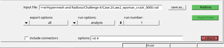
3) We run the simulation by going to the analysis module and clicking on radioss option with the starter file name as 'Law2_epsmax_crack_0000.rad' as shown in the image given below.
4) We go to Hyperview and import the file 'Law2_epsmax_crack.h3d' then, then we check for contour plot on Von mises stress with simple average method. After running the von mises animation we see that the elements in the plate the elements get cracked and then deleted. When Ifail_sh= 1: (Default) Shell is deleted or cracked when D=∑Δεpεf≥1 for one integration point or layer. If Ixfem =1: failure element will be CRACKED. Damage advancement Dadv=1 is present only when Ixfem is active. The animation as shown below.
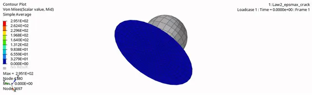
The max von mises stress was found out to be 295.1 MPa.
5) We look out for the energy error and mass error in 'Law2_epsmax_crack_0001.out' in the form of the text editor as shown in the image given below.
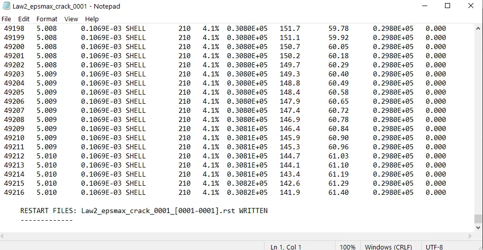
Energy Error: 4.1%
Mass Error: 0
Elapsed Time: 117.08 secs
No of Cycles: 49217
6) We then, proceed to plot the graphs the results with the help of Hypergraph 2D. We plot graphs for all the energies which include internal energy, kinetic energy and total energy. We don't plot graph for hourglass energy since we are using recommended shell formulation properties. The plots are shown in the images given below.
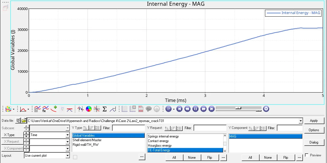
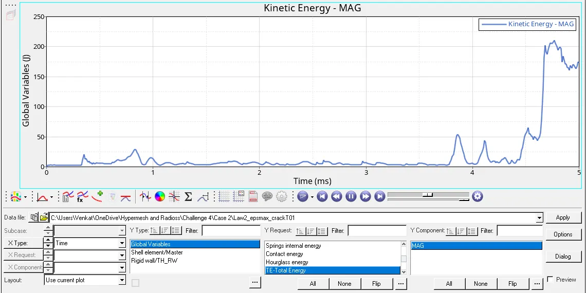
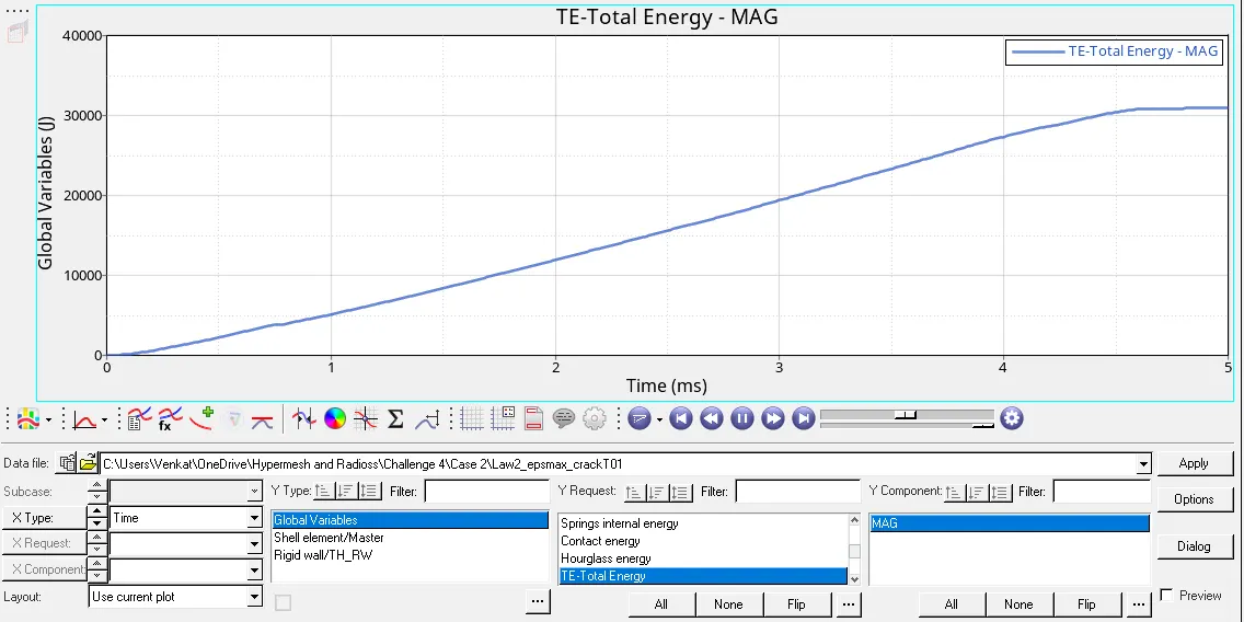
7) We see that in the internal energy plot the oscillating region is called the Strain Hardening Process. Beyond this region due to High Elongation loads it will undergo plastic strain followed by severe plastic strain and finally fails. The difference between the CASE1 and CASE2 is the direct deletion of the plate element and the crack advancement leading to the deletion has been observed.
3. Case-3:
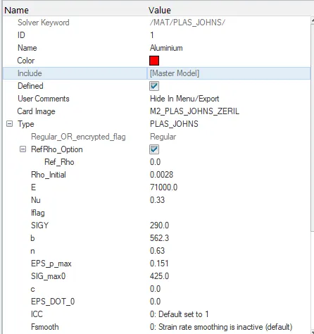
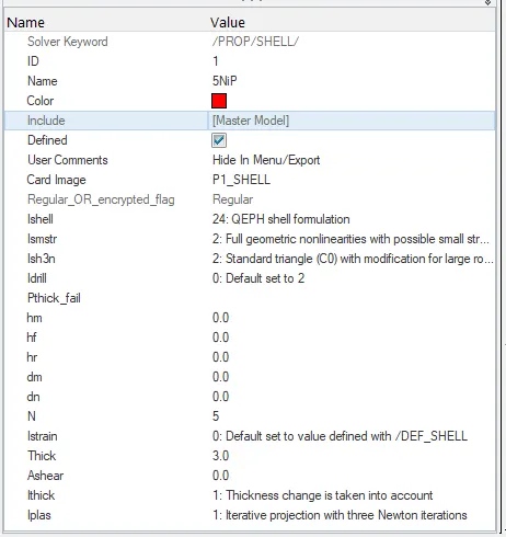
1) In case 3, we run the simulation with recommended properties, default material parameters and we delete the 'FAIL_JOHNSON' failure card.
2) We first import the rad file 'FAILURE_JOHNSON_0000.rad' and we run the simulation with default material and shell properties also we delete the 'FAIL_JOHNSON' failure card as shown in the images given below.
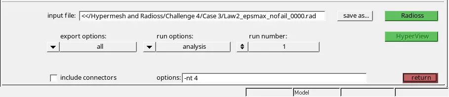
3) We run the simulation by going to the analysis module and clicking on radioss option with the starter file name as 'Law2_epsmax_nofail_0000.rad' as shown in the image given below.
4) We go to Hyperview and import the file 'Law2_epsmax_nofail.h3d' then, then we check for contour plot on Von mises stress with simple average method. After running the von mises animation we see that the elements in the plate the elements get deleted as shown in the animation given below.
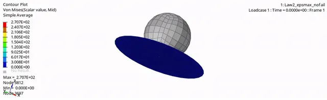
The max von mises stress was found out to be 270.7 MPa.
5) We look out for the energy error and mass error in 'Law2_epsmax_nofail_0001.out' in the form of the text editor as shown in the image given below.
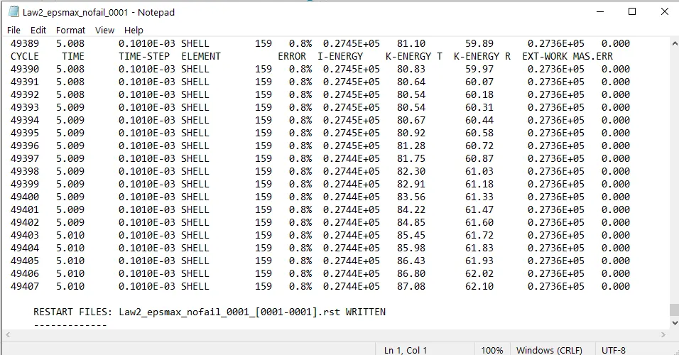
Energy Error: 0.8%
Mass Error: 0
Elapsed Time: 110.04 secs
No of Cycles: 49408
6) We then, proceed to plot the graphs the results with the help of Hypergraph 2D. We plot graphs for all the energies which include internal energy, kinetic energy and total energy. We don't plot graph for hourglass energy since we are using recommended shell formulation properties. The plots are shown in the images given below.
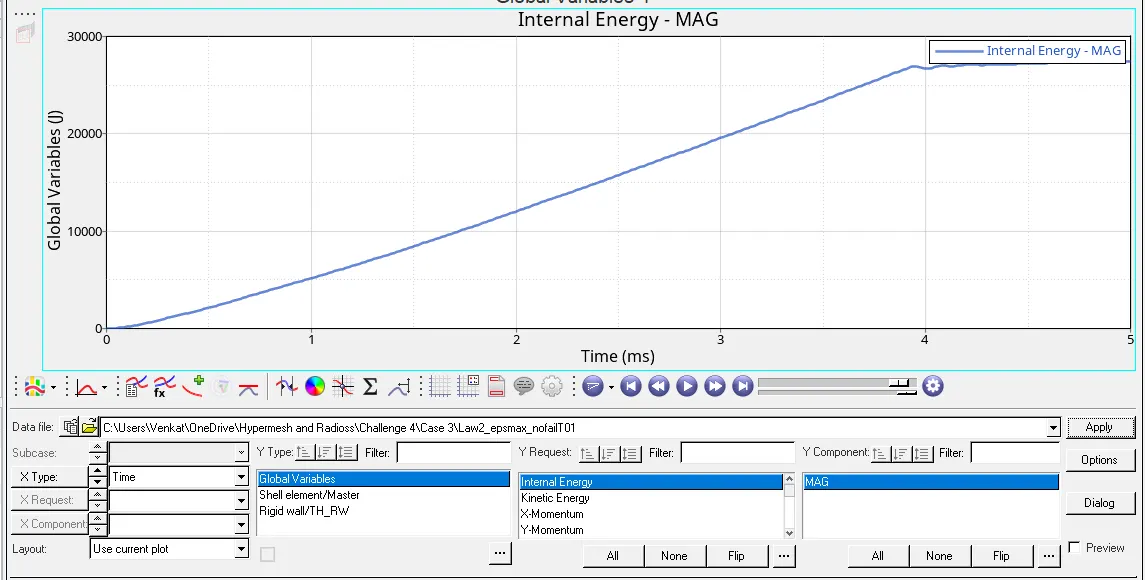
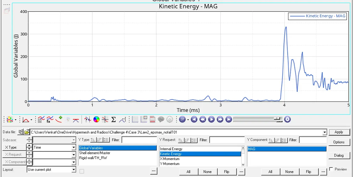
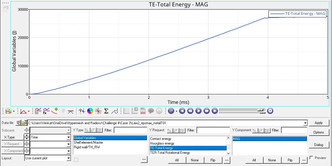
7) In case 3 the internal energy graph the energy increases upto 4ms but after that due to Strain-hardening process the internal energy values oscillates. The Kinectic energy graph gives only small spikes which indicate that the elements are getting deleted once reaching the maximum Strain rate of 15%. Case 3 and Case 1 are similar without any crack formation.
4. Case-4:
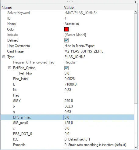
1) In case 4, we run the simulation with recommended properties, default material parameters and we remove the value of EPS_p_max in the material card.
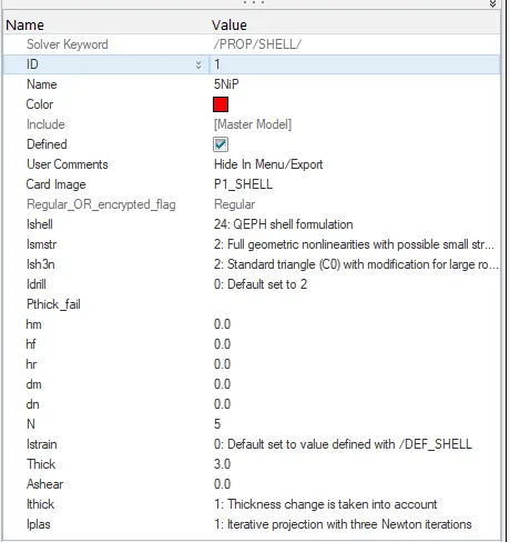
2) We first import the rad file 'FAILURE_JOHNSON_0000.rad' and we run the simulation with default material and shell properties also we remove the value of EPS_p_max in the material card as shown in the images given below.
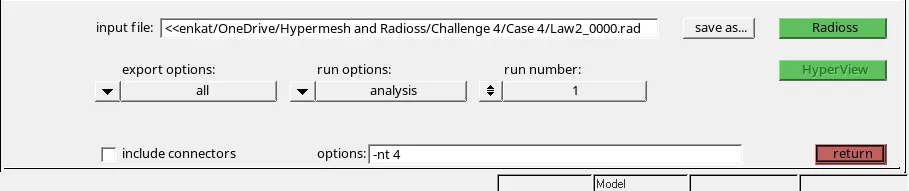
3) We run the simulation by going to the analysis module and clicking on radioss option with the starter file name as 'Law2_0000.rad' as shown in the image given below.
4) We go to Hyperview and import the file 'Law2.h3d' then, then we check for contour plot on Von mises stress with simple average method. After running the von mises animation we see that the elements in the plate the elements do not get deleted and crack propagates till the end as shown in the animation given below.
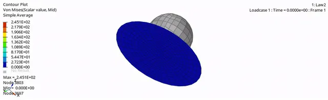
The max von mises stress was found out to be 245.1 MPa.
5) We look out for the energy error and mass error in 'Law2_0001.out' in the form of the text editor as shown in the image given below.
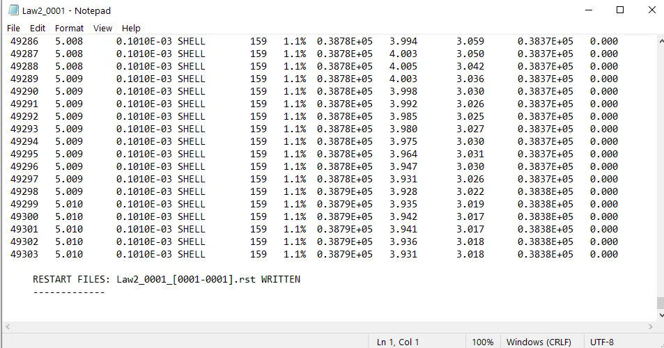
Energy Error: 1.1%
Mass Error: 0
Elapsed Time: 118.05 secs
No of Cycles: 49304
6) We then, proceed to plot the graphs the results with the help of Hypergraph 2D. We plot graphs for all the energies which include internal energy, kinetic energy and total energy. We don't plot graph for hourglass energy since we are using recommended shell formulation properties. The plots are shown in the images given below.
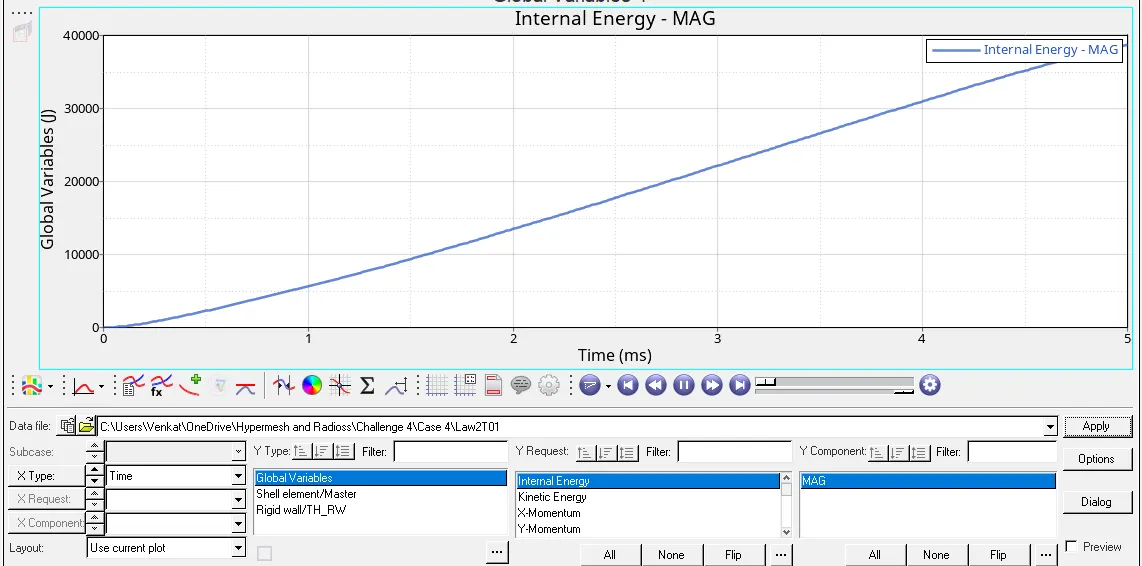
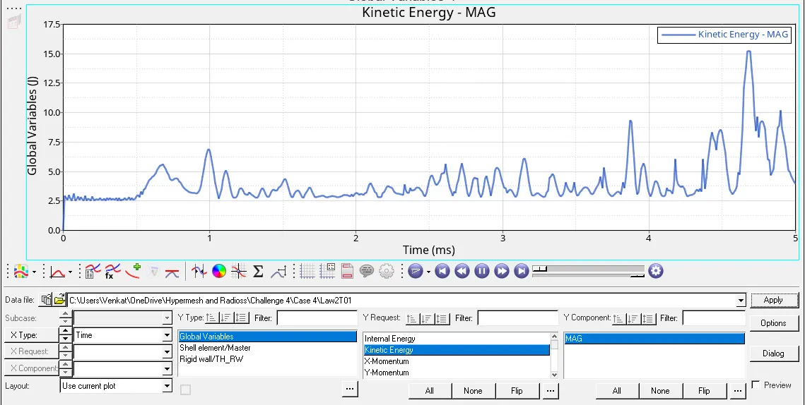
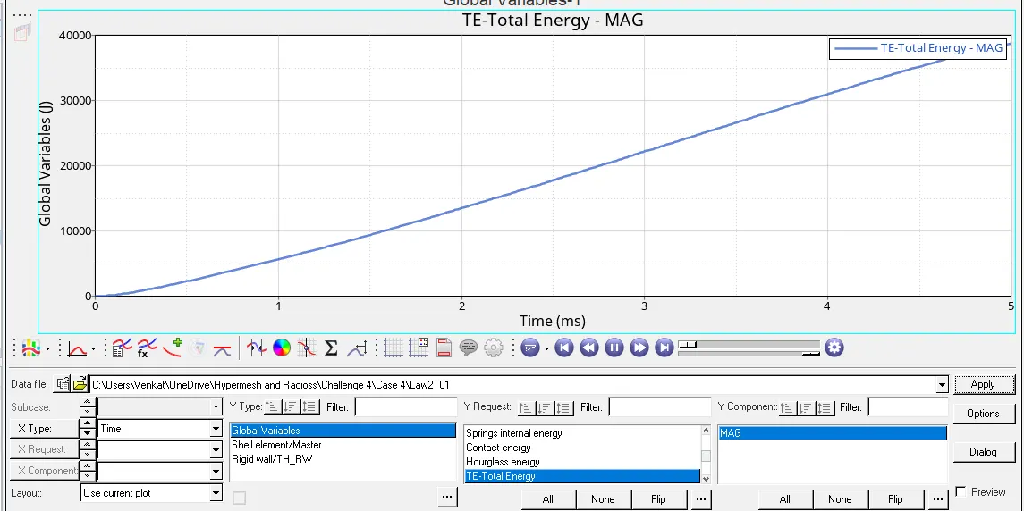
7) EPS_p_max is deleted so there is no plastic strain hardening. So the Internal Energy has an exponential growth since the element are only stretched till plastic limit.
5. Case-5:
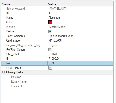
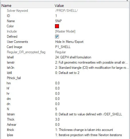
1) In case 5, we run the simulation with recommended properties, default material parameters and we change the card image to 'M1_ELAST' which defines an isotropic, linear elastic material using Hooke’s law in the material card.
2) We first import the rad file 'FAILURE_JOHNSON_0000.rad' and we run the simulation with default material and shell properties also we change the card image to 'M1_ELAST' in the material card as shown in the images given below.
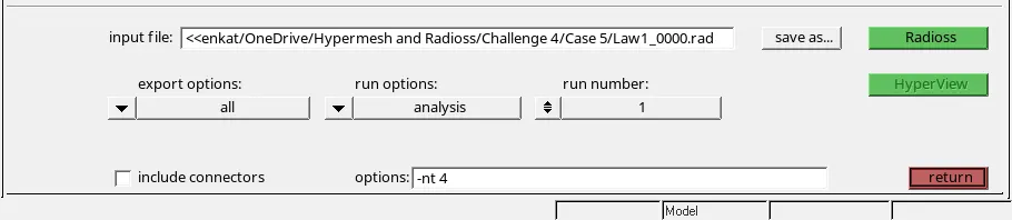
3) We run the simulation by going to the analysis module and clicking on radioss option with the starter file name as 'Law1_0000.rad' as shown in the image given below.
4) We go to Hyperview and import the file 'Law1.h3d' then, then we check for contour plot on Von mises stress with simple average method. After running the von mises animation we see that the elements in the plate the elements do not get deleted and crack too doesn't propagate till the end because the material is elastic as shown in the animation given below.
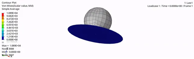
The max von mises stress was found out to be 10890 MPa.
5) We look out for the energy error and mass error in 'Law1_0001.out' in the form of the text editor as shown in the image given below.
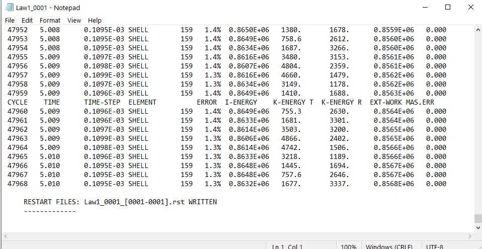
Energy Error: 1.3%
Mass Error: 0
Elapsed Time: 109.11 secs
No of Cycles: 47969
6) We then, proceed to plot the graphs the results with the help of Hypergraph 2D. We plot graphs for all the energies which include internal energy, kinetic energy and total energy. We don't plot graph for hourglass energy since we are using recommended shell formulation properties. The plots are shown in the images given below.
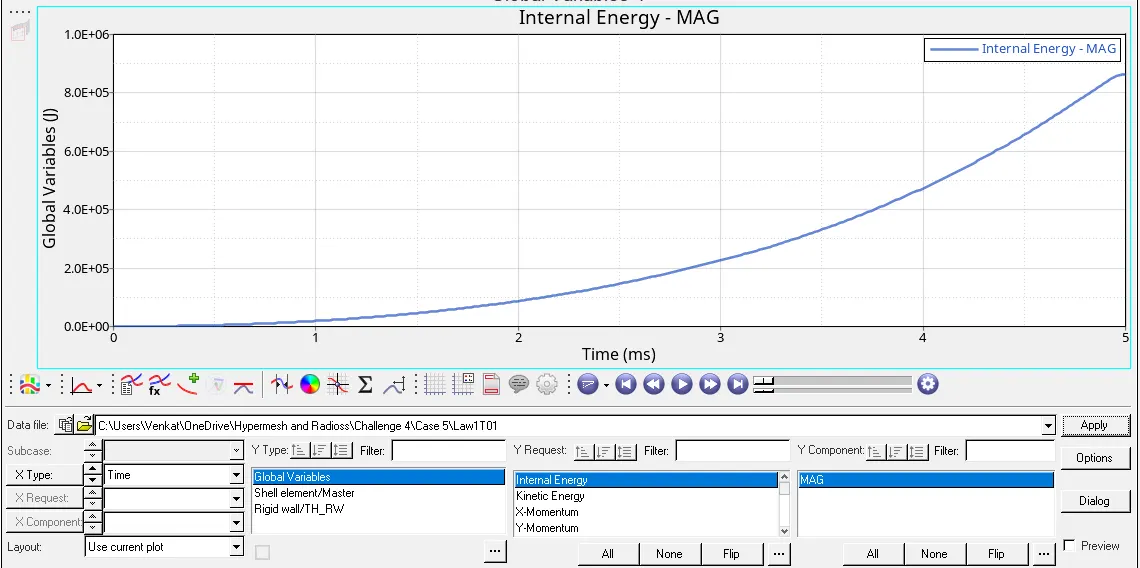
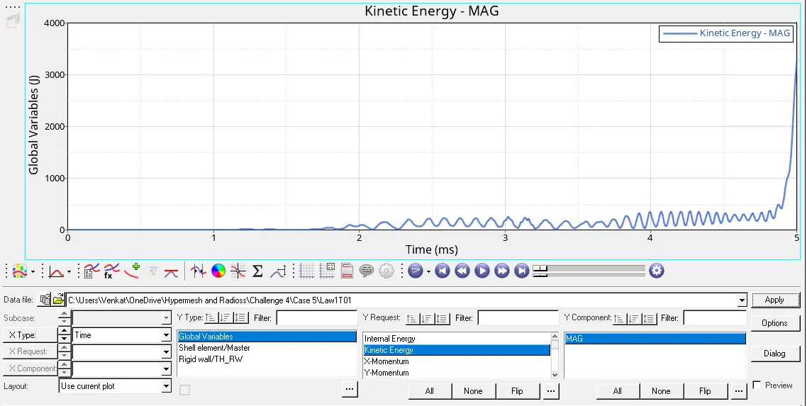
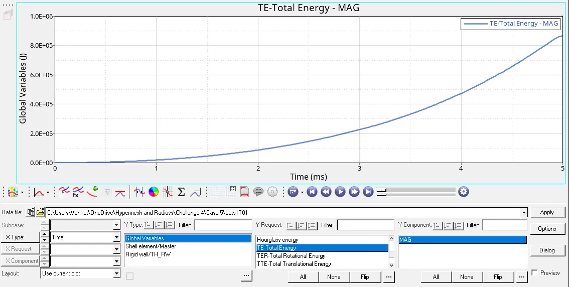
7) As the Material is linearly elastic or purely elastic there is no plastic strain as we see the internal energy plot. It just stretches and retakes it's shape when the load is retrieved.
6. Case-6:
1) In case 6, we run the simulation with recommended properties, default material parameters and we run it with default parameters.
2) We first import the rad file 'Law27_0000.rad' and we run the simulation with default material and shell properties also we run it with default parameters as shown in the images given below.
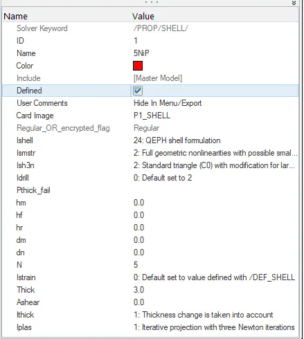
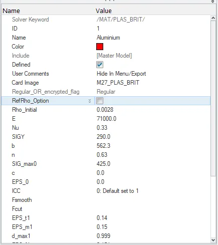
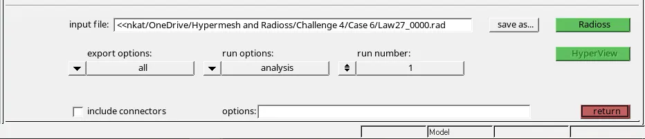
3) We run the simulation by going to the analysis module and clicking on radioss option with the starter file name as 'Law27_0000.rad' as shown in the image given below.
4) We go to Hyperview and import the file 'Law27.h3d' then, then we check for contour plot on Von mises stress with simple average method. After running the von mises animation we see that the elements in the plate the elements get deleted because the material is used as a brittle material as shown in the animation given below.
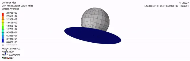
The max von mises stress was found out to be 287.5 MPa.
5) We look out for the energy error and mass error in 'Law27_0001.out' in the form of the text editor as shown in the image given below.
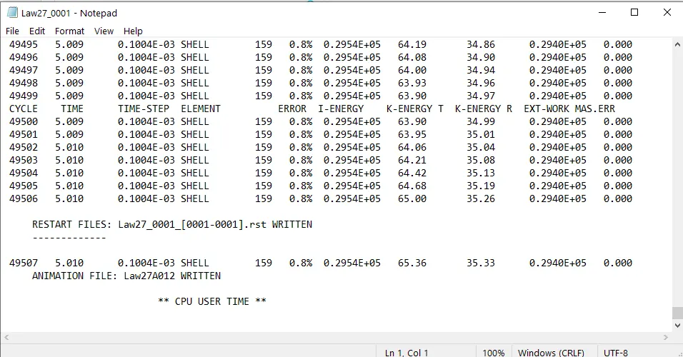
Energy Error: 0.8%
Mass Error: 0
Elapsed Time: 89.86 secs
No of Cycles: 49508
6) We then, proceed to plot the graphs the results with the help of Hypergraph 2D. We plot graphs for all the energies which include internal energy, kinetic energy and total energy. We don't plot graph for hourglass energy since we are using recommended shell formulation properties. The plots are shown in the images given below.
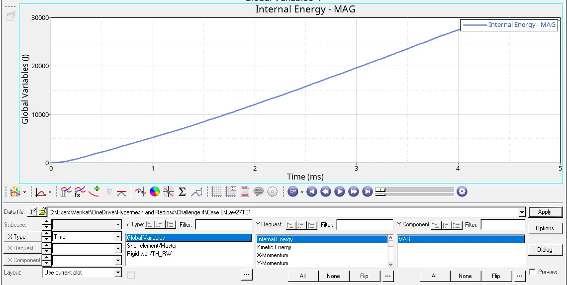
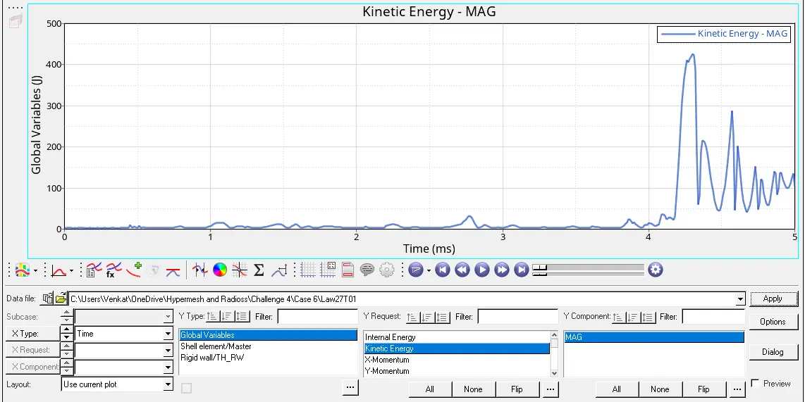
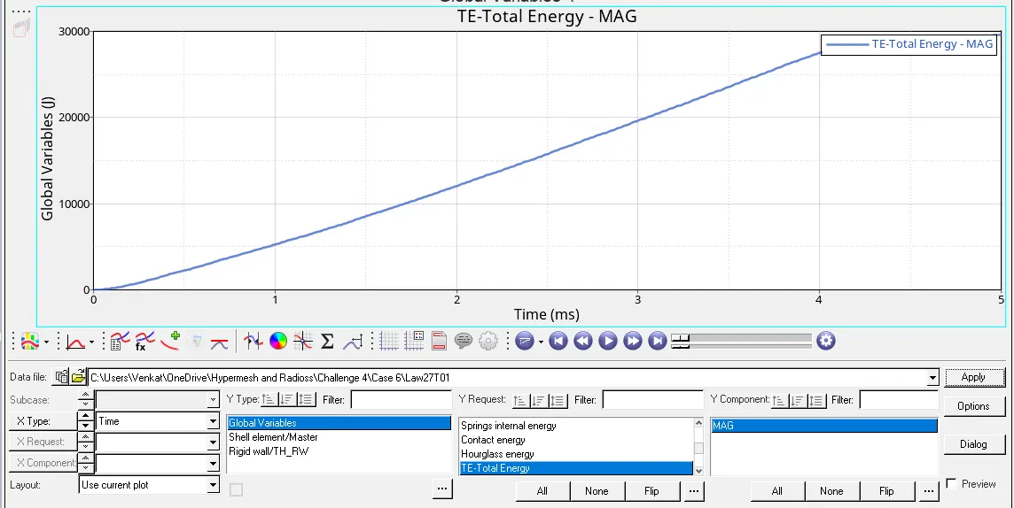
7) The element gets deleted when the Plastic strain reaches 0.15 because the material used here is a brittle material.
7. Case-7:
1) In case 7, we run the simulation with recommended properties, default material parameters and we run it with default parameters.
2) We first import the rad file 'FAILURE_JOHNSON_0000.rad' and we run the simulation with default material and shell properties also we change the card image to 'M36_PLAS_TAB' in the material card as shown in the images given below.
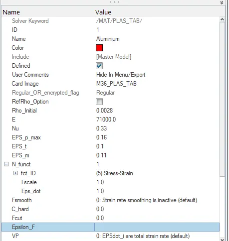
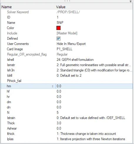
3)We also import the values in the material card according to the card that was given to us in the challenge as shown in the image given below.
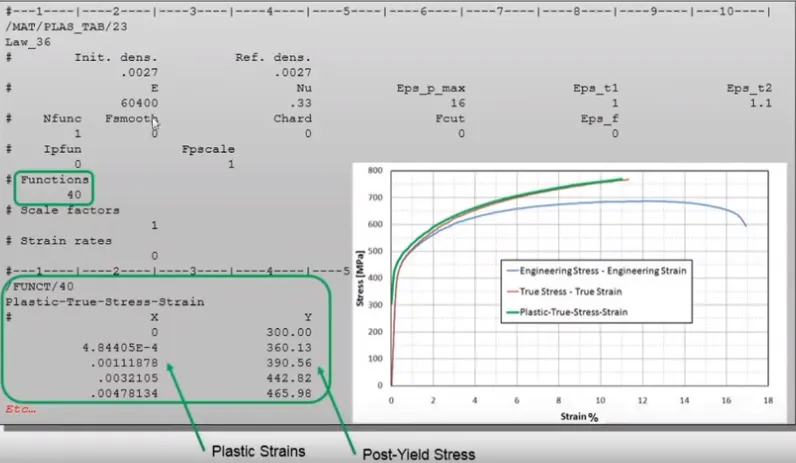
4) We have to also create curves by right clicking on the curves card with the input x and y values as mentioned in the above image. The created curve is shown in the image given below.
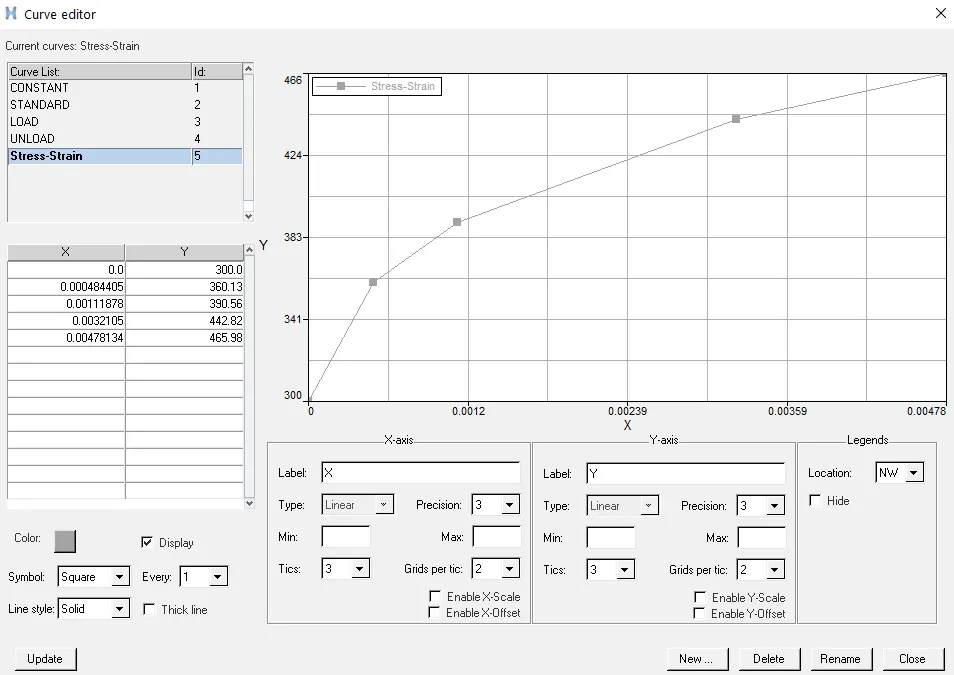
5) We run the simulation by going to the analysis module and clicking on radioss option with the starter file name as 'Law36_0000.rad'. We go to Hyperview and import the file 'Law36.h3d' then, then we check for contour plot on Von mises stress with simple average method. After running the von mises animation we see that the elements in the plate the elements get deleted because the material is undergoing user defined plastic strain hardening as shown in the animation given below.
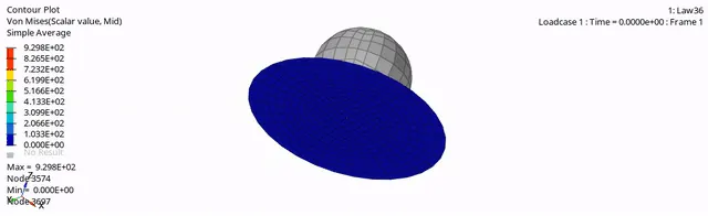
The max von mises stress was found out to be 929.8 MPa.
6) We look out for the energy error and mass error in 'Law36_0001.out' in the form of the text editor as shown in the image given below.
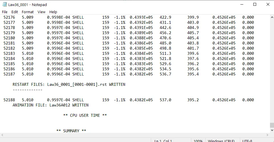
Energy Error:-1.1%
Mass Error: 0
Elapsed Time: 126.65 secs
No of Cycles: 52189
7) We then, proceed to plot the graphs the results with the help of Hypergraph 2D. We plot graphs for all the energies which include internal energy, kinetic energy and total energy. We don't plot graph for hourglass energy since we are using recommended shell formulation properties. The plots are shown in the images given below.
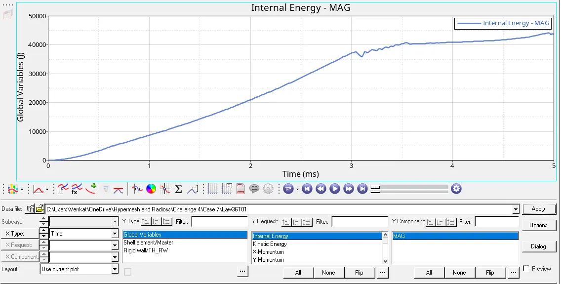
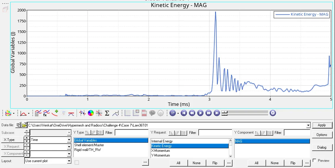
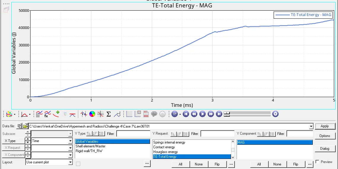
8) The element gets deleted when the Plastic strain reaches 0.16. Beyond this region due to High Elongation loads it will undergo plastic strain followed by severe plastic strain and finally fails.Work hardening is seen in these materials can be observed as seen in the Law2.
Results and Discussion:
Comparison of all 7 cases:
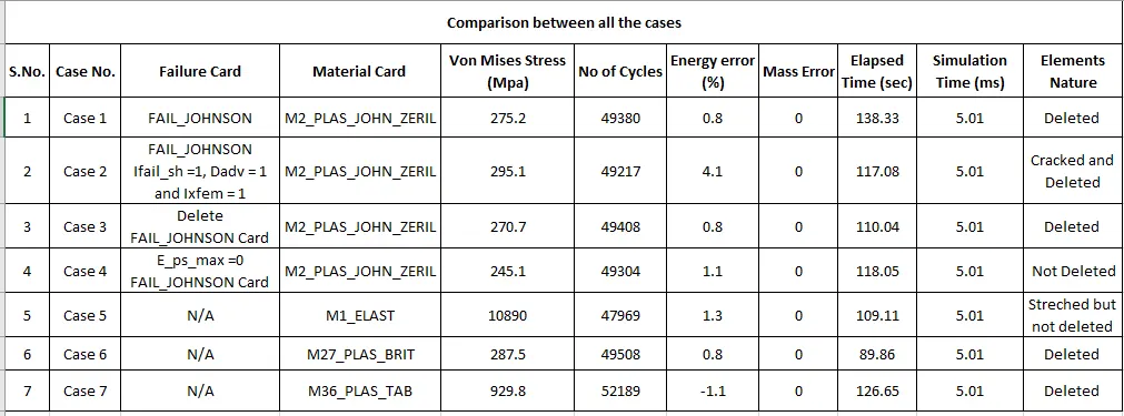
1)By comparing all the cases we can say that the energy errors that are obtained are very much acceptable i.e. the standard values can lie between -15 % to +5%.
2) The mass error on the other hand can be seen as acceptable because it is zero.
3) The no of cycles and elapsed time depend on the type of Material Law used in the simulation. The simulation time for all the cases remains 5.01 ms.
4) From the above result, we can say that the Law 36 which is an isotropic elasto-plastic material that uses user-defined functions for the work-hardening portion of the stress-strain curve for different strain rates can be used for on field scenario's.
Conclusion:
1) We learnt about different Material Laws used in the industry by performing this plate and ball experiment with different material laws such as Law1, Law2, Law27 and Law36.
2) We simulated all the cases that were provided to us. We also plotted 2D graphs and Contour Plots using Hyperview and Hypergraph 2D.
3) We have also tabulated results and have also mentioned the nature of elements after simulation.
3) We have said Law 36 could be used for on field senario's involved in these kind of failure process.
Model Link:
https://drive.google.com/file/d/1Gtr97SthS19YewZJTLcFD9tPCRyrNR41/view?usp=sharing