Simulation of Frontal Crash of Dodge Neon BIW model using Radioss

Aim:

1. To perform Frontal Crash for Neon car BIW Model by initially setting up with the following parameters:

1) Checking the unit system and following either of these unit systems[Mg mm s] or [Kg mm ms].

2) Creating appropriate Type 7 interface, inputting value of friction=0.2 and also inputting other recommended parameters.

3) Checking for penetrations and intersections and if found fixing them.

4) Correcting rigid bodies if any issues.

5) Create rigid wall with friction 0.1.

6) Using added masses to reach target weight 700kg while getting CG about the required range.

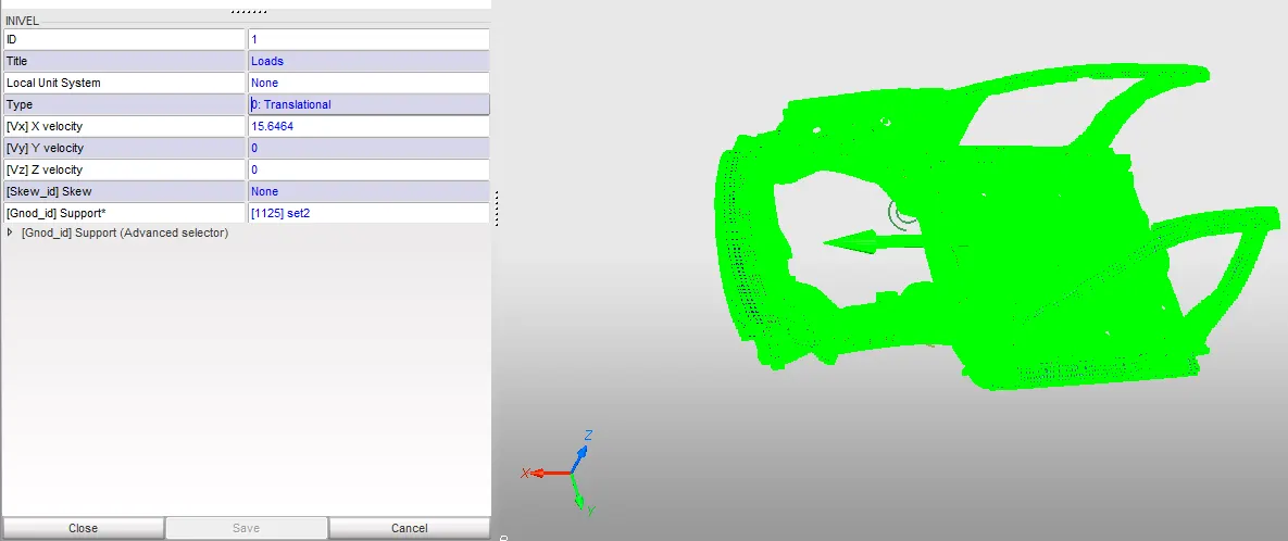
7) Keeping the Initial velocity at 35 mph=15.6464 mm/ms.

8) Using the model checker to ensure good quality.

9) Checking the timestep and runtime of the model.

2. After running the simulation we have to lookup for the following output requests:

1) Sectional force in the rails at location of indicated node 174247.

2) Axial force received on the rails from bumper.

3) Shotgun cross sectional forces.

4) A pillar cross section.

5) Acceleration curve received on the accelerometer at base of B pillar (on B pillar rocker).

6) Intrusions on the dash wall 66695,66244.

7) Energies plotting and notice difference in them.

Theory:

The model given to us is Dodge Neon BIW model with which we have to perform Frontal crash. The Frontal Crash is done by creating a rigid wall in front side i.e. the bumper side of the car.

Procedure:

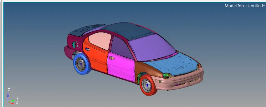
1) We have been given the Neon Dodge full scale model as shown in the image given below.

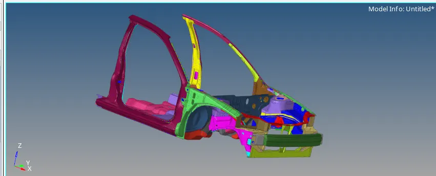
2) The reduced BIW model is given below and it is the one which considered for further analysis of the Frontal Crash.

Setting up the model:

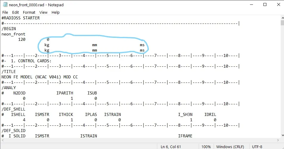
1) We first check the unit system for the model by opening the 0.rad file in text editor as shown in the image given below. We find that the unit system is in [Kg mm ms], therefore we can proceed for further process.

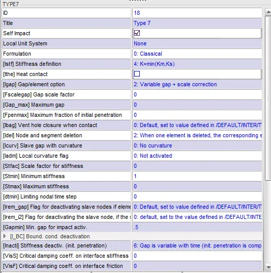
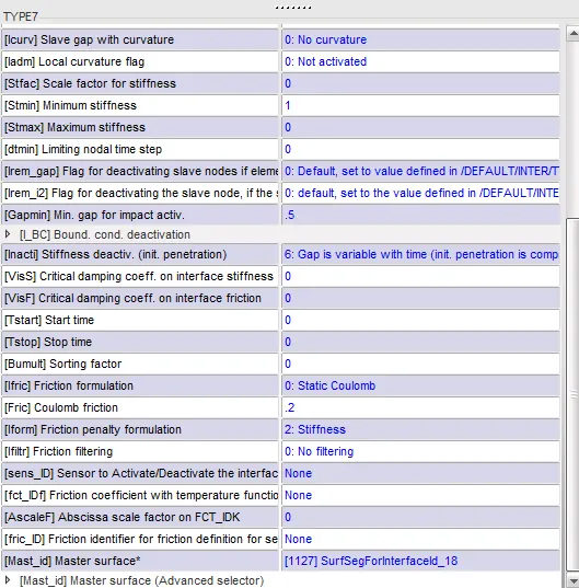
2) We create a Type 7 contact interface by selecting the masters nodes, the slave nodes are not selected since its a self impact. The value of friction i.e. 0.2 is inputted and other recommended parameters are also inputted as shown in the image given below.

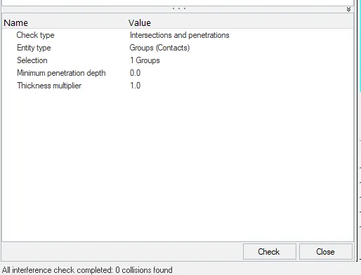
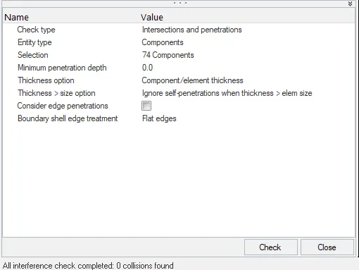
3) We then proceed to check for any penetrations and intersections in the model. We run the penetration checker for both groups(contacts) and components, we find that there no penetrations or intersections in the model as shown in the image given below.

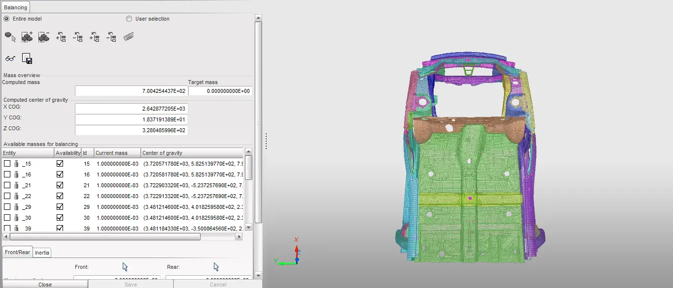
4) We then check all rigid bodies and find if there issues in it, we find that there are no issues in it. After that, we do a comparison for the full scale model and reduced model for correct location of the COG. The COG is found and then we correct using the mass balancing option in the Hypercrash. We use addmass to add weight and finally we bring the weight of the body to 700 kg and the COG moves backward to location were the driver's seat is located. The location of COG is given in the image below.

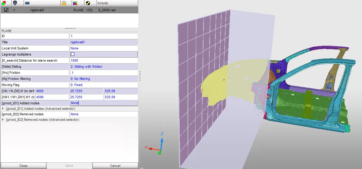
5) We also create rigid wall with sliding friction=0.1 so that the car can hit the wall on giving initial velocity.

6) We input the value of initial velocity by creating a card called Inivel and we input the value of initial velocity as 35 mph=15.6464 mm/ms in the positive X direction were the rigid wall is located as shown in the image given below.

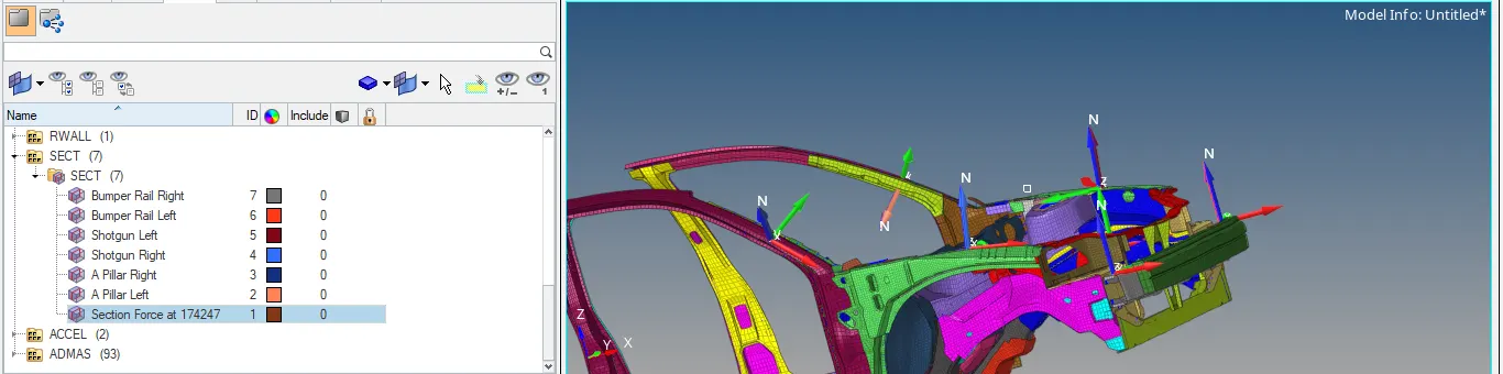
7) We create sections in the model as mentioned in the aim, for that we create moving frames then we create section, then we mention the value of N1,N2 & N3 by selecting the nodes after we select the Frame we created and finally we select the elements that are needed to part of the section. Then we create time history files for them so that the output results could be obtained and they can be plotted using the Hypergaph 2D. The created sections are shown in the image given below.

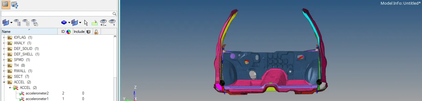
8) After that, we create Accelerometer on the B pillar rocker, so that we can measure the acceleration that is recieved on B pillar. The Accelerometer created is shown in the image given below.

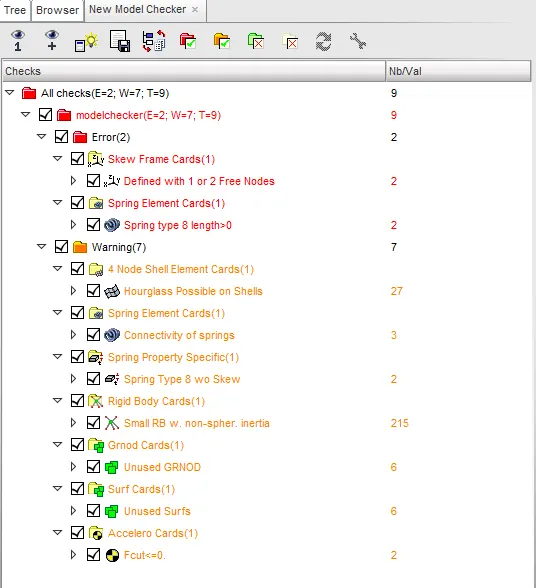
9) We then run the model checker so as to find whether there are any errors or warnings in the model so that we can clear them before running the simulation. We find there are 7 warnings and 2 errors as shown in the image given below.

10) We then, rectify the errors and warnings one by one manually and finally we obtain 0 errors and warnings.

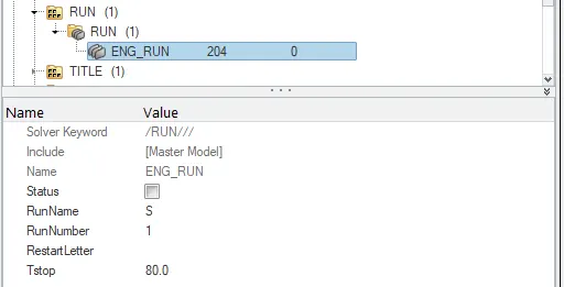
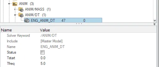
11) Before, we run the simulation we have to check the timestep and runtime of the model. We, find that the runtime and timestep are correct i.e. 80 ms and 5 as shown in the images given below. Therefore, we can proceed to run the model in the Radioss.

12) We then, go the Analysis module and go to Radioss option then, we save the Starter File wherever required and then we run the simulation as shown in the image given below.

Simulated model results:

1) After running the simulation, we look out for the energy error and mass error in '0001.out' in the form of the text editor as shown in the image given below.

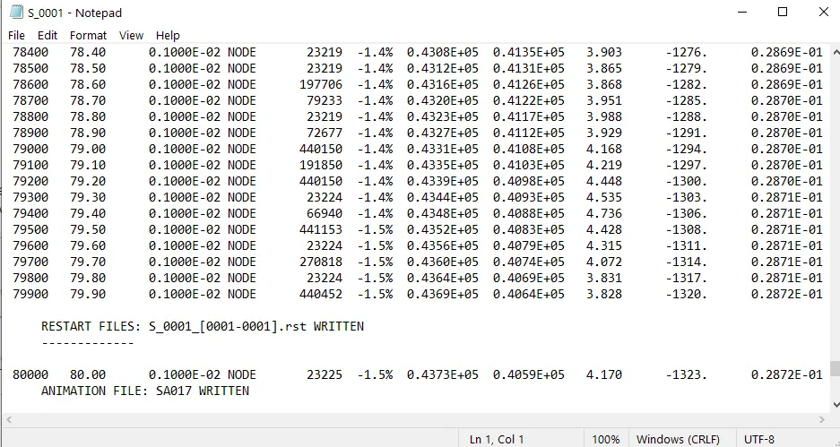
Energy Error: -1.5%

Mass Error: 0.0287 kg

No of Cycles: 80,001

2) We go to Hyperview and import the file '.h3d' then, we check for contour plot on Von mises stress with simple average method and Displacement in the form of animations as shown below.

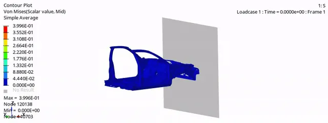
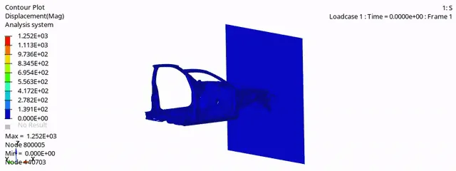
Max Von Mises Stress: 0.3996 GPa

Max Displacement: 1252 mm

3) We then, proceed to plot the graphs the results with the help of Hypergraph 2D.

4) We plot graphs for all the energies which include internal energy, kinetic energy, Contact energy, Hourglass energy & total energy are shown in the image given below.

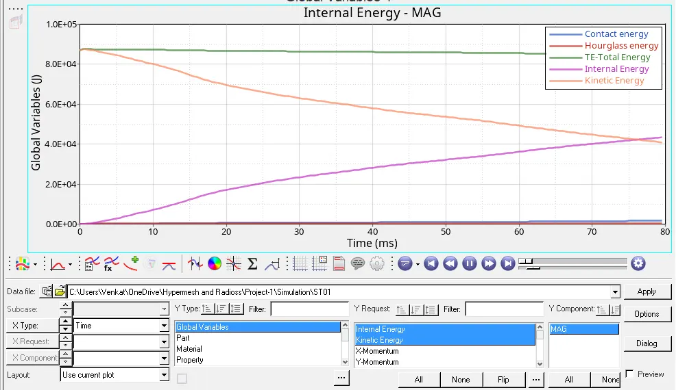
In this plot, we can see that the Internal energy increases to almost 45,000 J at the end of simulation, Kinectic Energy decreases from 88,000 J to 40,000 J at the end of the simulation, the Hourglass energy & Contact energy remain at 0 J for all the time since we use the recommended shell formulations for all the components & there is also no contact between till the completion of the simulation and finally, the Total Energy also remains constant i.e. at 88,000 J till the end of simulation since there is no significant energy loss.

5) We plot graph for rigid wall forces as shown in the image given below.

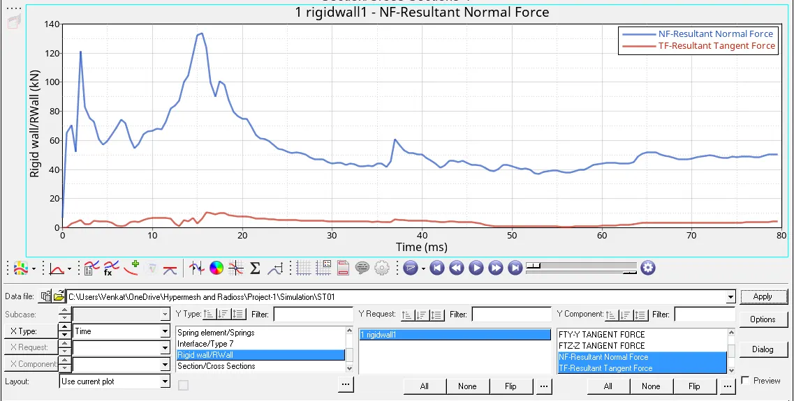
In this plot, we can see that at the event of crash the rigid wall resultant normal forces are more i.e. at 135KN , then it decreases since the crash event is finished .

6) We plot graphs for all the cross sectional forces as shown in the images given below.

1. Sectional force in the rails at location of indicated node 174247.

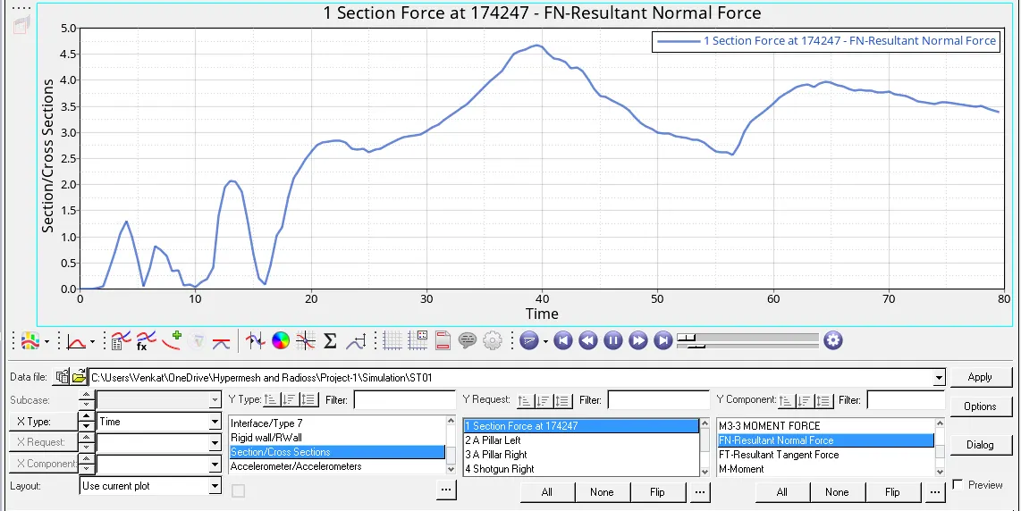
The sectional forces are the highest at the around 40 ms with 4.75 KN and it decreases for some time then, again there is a sudden increase at 65 ms i.e 4 KN.

2. Shotgun cross sectional forces.

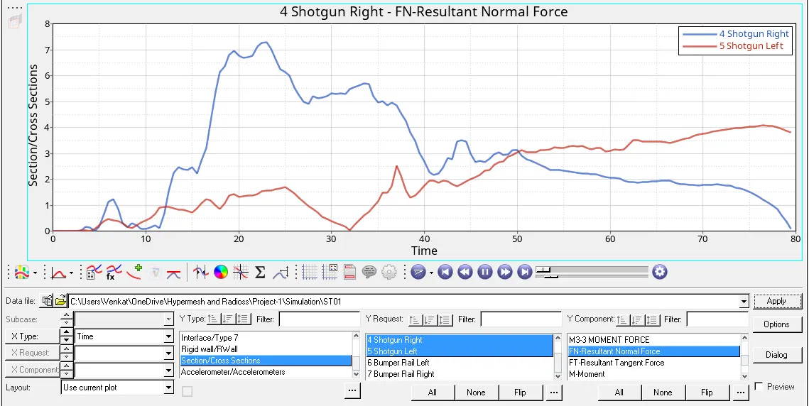
The shotgun region forces for the left side is maximum at 23 ms i.e. 7.5 KN and then decreases with respect to time, whereas in the right side the maximum value of force is recorded at the end of the simulation i.e. 80 ms the force value is 4 KN

3. A pillar cross section.

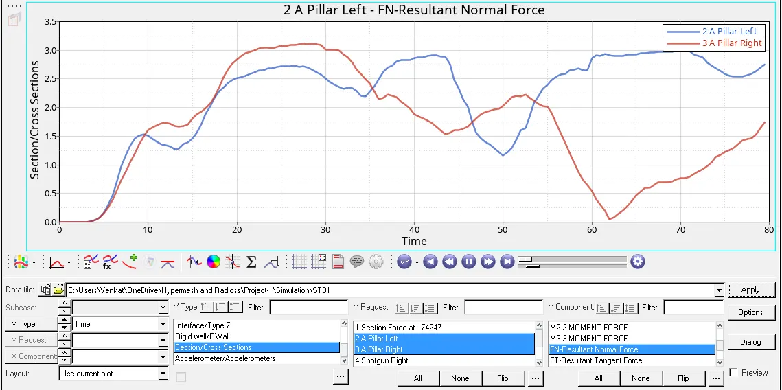
The A pillar forces for both increase gradually till 25 ms here the highest value of force is recorded for the right side of the A pillar i.e. 3.6 KN. The highest value of left side part is recorded at 70ms i.e. 3 KN.

7) We plot graphs for Axial force received on the rails from bumper as shown in the image given below.

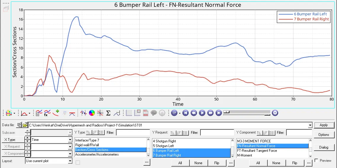
The axial for the left side rail is highest at 14 ms i.e. 16.5 KN and for the right side it is highest at 7 ms i.e. 9 KN. The bumper forces are high at the start of the crash since the bumper hits the rigid wall first after that only the body deformes.

8) We plot graphs for Acceleration curve received on the accelerometer at base of B pillar (on B pillar rocker) as shown in the image given below.

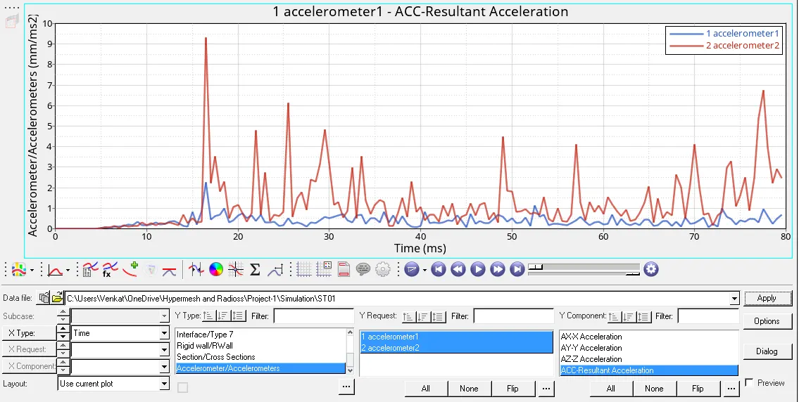
The accelerations with 2 accelerometers placed on the Bpillar rockers on either sides of the BIW model are highest at around 17 ms i.e. 9mm/ms^2 on left side and 2 mm/ms^2 on the right side. The acceleration curve has a lot of spikes since deformation of body and its acceleration keeps on increasing and decreasing.

9) We finally, plot graphs for Intrusions on the dash wall for node nos 66695 & 66244 as shown in the image given below.

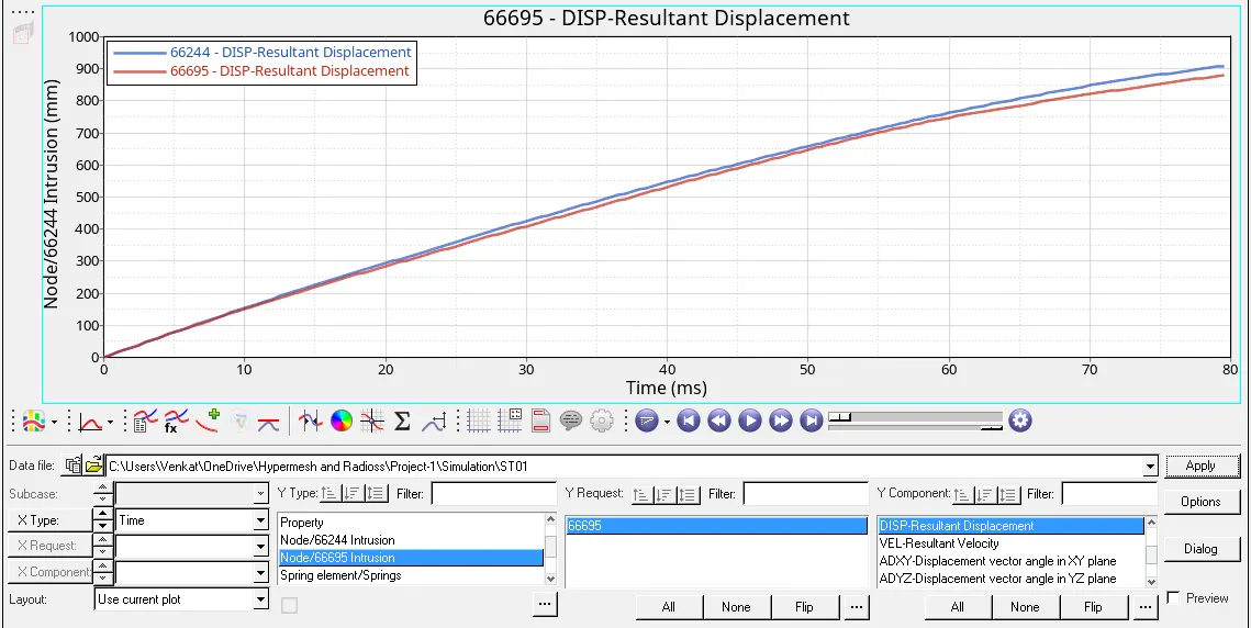
The node no 66244 has a displacement of 900mm at the end of the simulation and for node no 66695 has a displacement of 875 mm at the end of the simulation. The intrusions are increasing linearly since, the deformation occurs in a linear manner.

Conclusion:

1) We have set-up the model for Frontal Crash according to the given parameters in the aim.

2) We have checked for penetrations and intersections in the model.

3) We have also used the model checker to find errors and warnings in the model and then rectify them manually one by one.

4) We have run the simulation and we have noted that the energy error and mass errors are within the controlled limit.

5) We seen the animations for displacement and von mises stresses in the Hyperview.

6) We have also plotted the graphs for energies, cross sections, intrusions, accelerations and rigid wall forces at all the points or sections that are given in the aim using Hypergraph 2D.

Model Link:

https://drive.google.com/file/d/1fbact_QLjWPxkIpKuXmpK2AIA65xGkO3/view?usp=sharing