Crash Box Simulation using LS-DYNA

Aim:

that crashes onto the rigid wall.

2) To maintain the gm-mm-ms unit system and provide an initial velocity of 50 kmph to the crash box.

3) To get the output contour animation and other plots upon running the simulation.

Procedure:

Importing the Model:

1) We first open the LS Prepost software and import the keyword file (.k file).

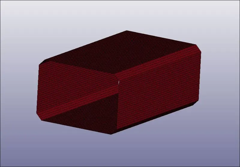
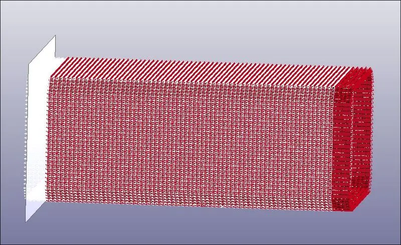
2) The keyword file consists of a crash box as shown in the image given below.

Assigning Material:

3) We then, assign the material properties to the crash box. We will use Steel Material Properties For the Crash Box. Although many material models exist for metals, one of the most robust models is *MAT_024 or *MAT_PIECEWISE_LINEAR_PLASTICITY. This material model is the standard workhorse and is the recommended starting point for elastic-plastic simulation of metals and general plastics since it can also handle viscoelastic behavior (i.e., strain-rate dependency). And for defining this material we are using MAT_024 (MAT_PIECEWISE_LINEAR_PLASTICITY), This is Material Type 24, which is an elastoplastic material with arbitrary stress.

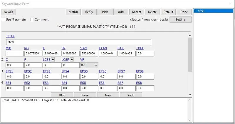
Here,

1. MID: Material identification. A unique number or label not exceeding 8 Characters must be specified.
2. RO: Mass density.
3. E: Young’s modulus.
4. PR: Poisson’s ratio.
5. SIGY: Yield stress.
6. ETAN: Tangent modulus, ignored if (LCSS.GT.0) is defined.

Assigning Sections:

4) Section Creation Define the section Properties for different elements. Since there is only one component in this model which is a shell element, we use SECTION_SHELL. We also parallelly assign section properties to a 1.5 mm thickness crash box as well.

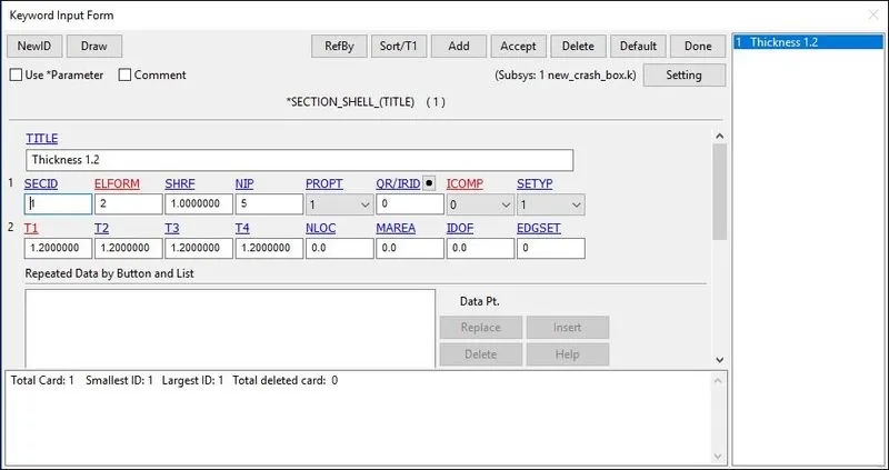
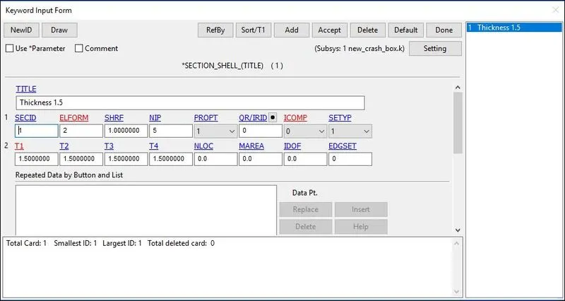
Here,

1. SECID: Section ID. SECID is referenced on the *PART card. A unique Number or label must be specified.
2. ELFORM: Element formulation options.= 2 Belytschko-Tsay
3. SHRF: Shear correction factor which scales the transverse shear stress.= 1
4. NIP: Number of through-thickness integration points = 5
5. T1: Shell thickness = 1.2 mm and 1.5 mm

Assigning Materials and Sections to Parts:

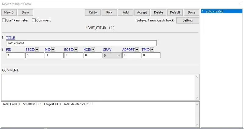
5) The Material and Section keyword is created and now they have to be assigned to the respective Part.

Contact Creation:

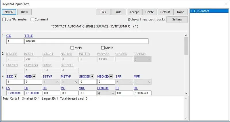
6) In case of crash scenarios where the Crash box crashes into the rigid wall there is change crash box buckles and penetrates itself. So, it is recommended that AUTOMATIC_SINGLE_SURFACE has to be considered. The only Slave can be defined in this type of contact.

Here,

1. SSID: Slave SetID, it is defined using part type.
2. MSID: Master SetID, it is also defined using part type.
3. SSTYP: Slave Set Type, it is selected according to the part.
4. MSTYP: Master Set Type, it is also selected according to the part.
5. FS: Static Friction = 0.2
6. FD: Dynamic Friction = 0.15

Rigid Wall Creation:

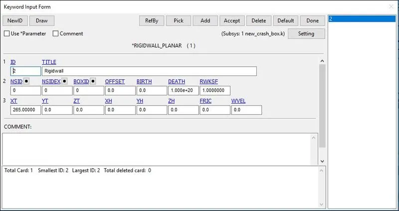
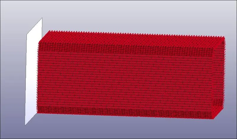
7) A *RIGIDWALL_PLANAR keyword has been created on where the box impacts. The Rigid wall was positioned 265mm away from the crash box. The direction of the normal of the generated rigid wall should be in the opposite direction of the velocity.

Initial Velocity:

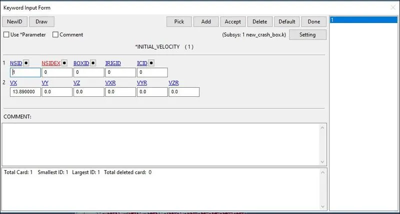
8) The Initial Velocity is defined to the mobile phone with the value of 13.89 mm/ms in a positive X direction which is towards the Rigidwall is added.

Here,

1. NSID: Node Set ID, we already created the node-set for the floor.
2. VX: Velocity along Translational X-axis.
3. VY: Velocity along Translational Y-axis.
4. VZ: Velocity along Translational Z-axis.
5. VXR: Velocity along Rotational X-axis.
6. VYR: Velocity along Rotational Y-axis.
7. VZR: Velocity along Rotational Z-axis.

Control Cards:

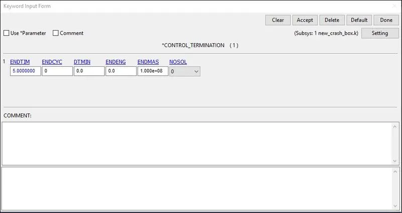
9) Control­_Termination is defined at what time the simulation ends or the end time of the simulation and it is set to 5 ms.

Here,

ENDTIM: It is the time at which the simulation ends.

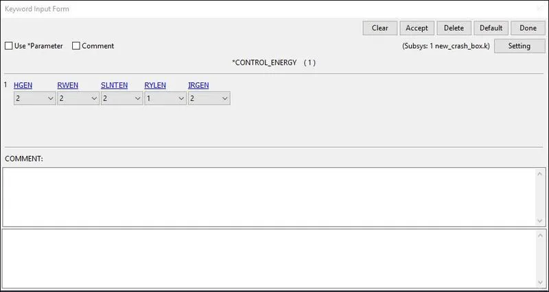
10) Control_Energy provides controls for energy dissipation options.

Here,

1. HGEN: Hourglass energy calculation option. Is set to 2 In Which hourglass energy is computed and included in the energy balance.
2. RWEN: Rigid wall energy dissipation option: Is set to 2 in Which energy dissipation is computed and included in the energy balance.
3. SLNTEN: Sliding interface energy dissipation option Since the Contact is Defined it is set to 2 so that energy dissipation is computed and included in the energy balance.

Database Creation:

11) BINARY_D3PLOT is defined as the frequency at which the animation file is to be created and is set to 0.1ms.

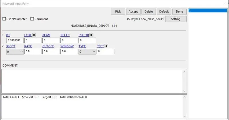
Here,

DT: Time-frequency at which the animation files should be printed.

12) One of the required outputs is Cross-sectional force at the middle of the crash box for this a DATABASE_CROSS_SECTION_PLANE.

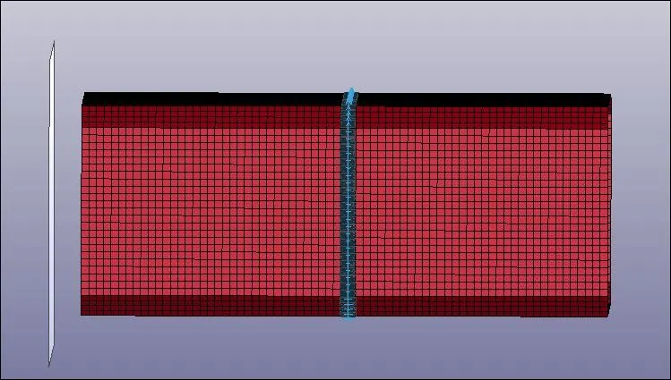
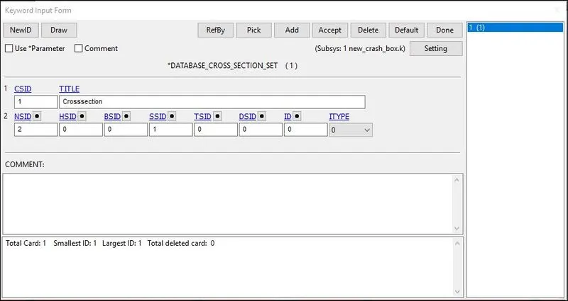
Here,

1. NSID: Node Set ID.
2. SSID: Shell Set ID.

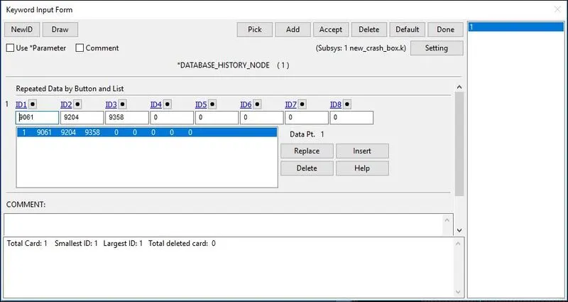
13) Three nodes were defined in the middle of the crash box to measure the acceleration using the DATABASE_HISTORY_NODE.

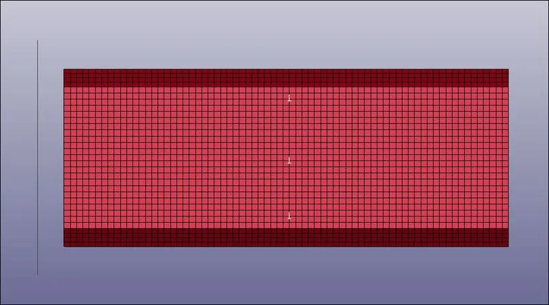
14) ASCII_option keyword is the output request in ASCII format, The following keywords are Activated.

1. ELOUT: Element Data
2. GLSTAT: Global Data
3. MATSUM: Material Energies
4. SLEOUT: Sliding Interface Energies
5. NODOUT: Nodal point data
6. SECFORC: Cross-section forces

Keywords:

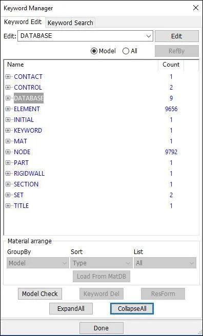
15) Finally, we have set up the simulation model and have a final look at our keyword manager which contains all the necessary parameters for running the simulation.

Model Check:

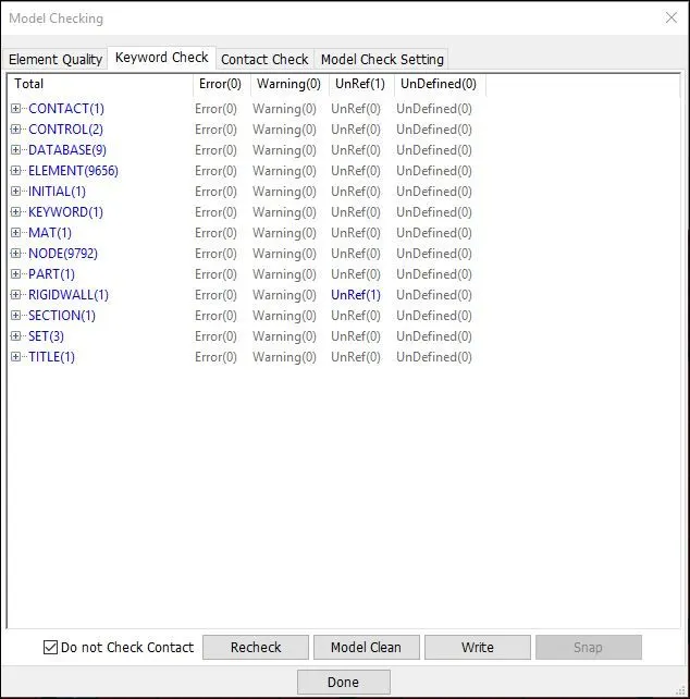
16) We perform model checking to find any errors or warnings present simulation model.

Results and Discussion:

1) We save the LS Dyna keyword file in a different folder and we go to the LS-Run Manager and run the simulation by importing the LS Dyna keyword file. The simulation finishes successfully with a normal termination.

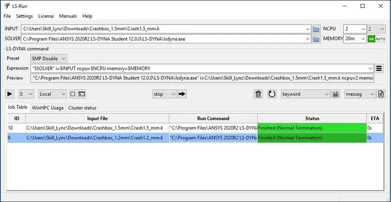
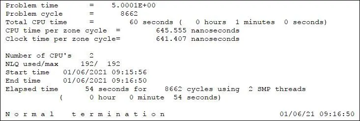
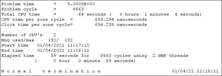
2) We then go to the lsrun.out file and open it with a text editor to see the time taken for both 1.2 mm and 1.5 mm crash boxes to complete the simulation.

Contour Animation:

3) We input the binary d3 plot keyword file and first we plot the contour animation for x and y directional stress for that we go to the Post-processing tab and click on the Fringe component. Then, we plot the X and Y stress under the stress tab for both 1.2 mm and 1.5 mm thickness crash boxes.

Crash box 1.2 mm:

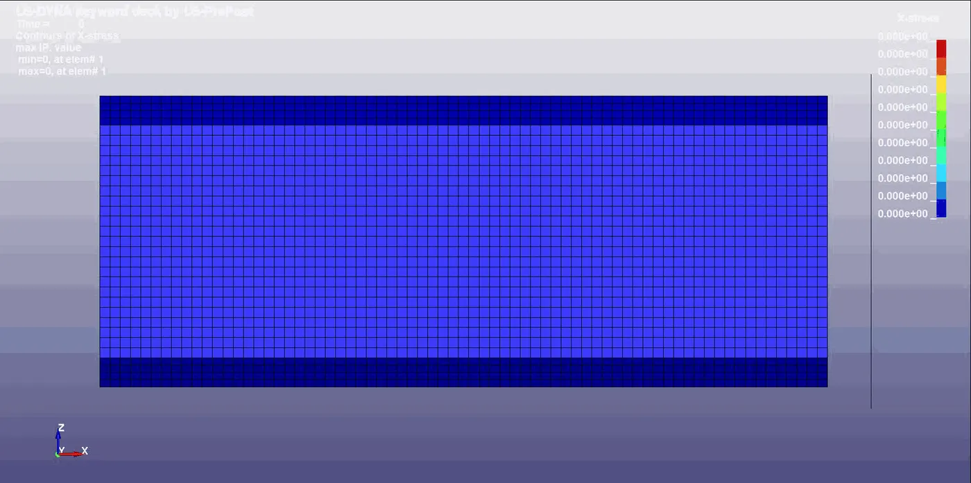
The min X directional Stress is found to be at -91.3576 MPa at element no 6960 and max X directional Stress is found to be at 275.416 MPa at element 7374.

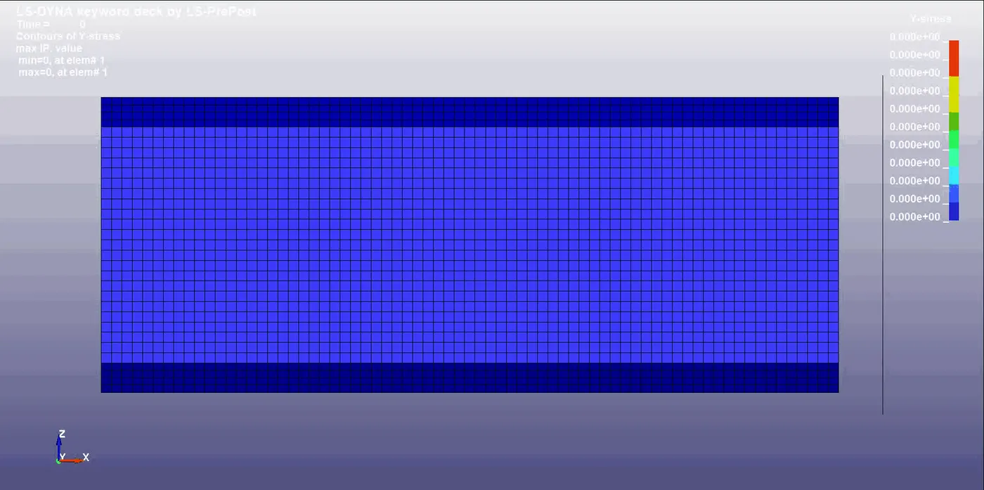
The min Y directional Stress is found to be at -161.688 MPa at element no 6311 and max Y directional Stress is found to be at 418.338 MPa at element 4291.

Crash box 1.5 mm:

The min X directional Stress is found to be at -423.28 MPa at element no 4469 and max X directional Stress is found to be at 316.319 MPa at element 7406.

The min Y directional Stress is found to be at -161.666 MPa at element no 6477 and max Y directional Stress is found to be at 428.183 MPa at element 6019.

4) We input the binary d3 plot keyword file again and we plot the contour animation for x and y directional strain for that we go to the Post-processing tab and click on the Fringe component. Then, we plot the X and Y strain under the S.rate tab for both 1.2 mm and 1.5 mm thickness crash boxes.

Crash box 1.2 mm:

The min X directional Strain is found to be at -1.00813 at element no 4658 and the max X directional Strain is found to be 0.934682 at element 6625.

The min Y directional Strain is found to be at -0.147018 at element no 6042 and the max Y directional Strain is found to be 0.129595 at element 5952.

Crash box 1.5 mm:

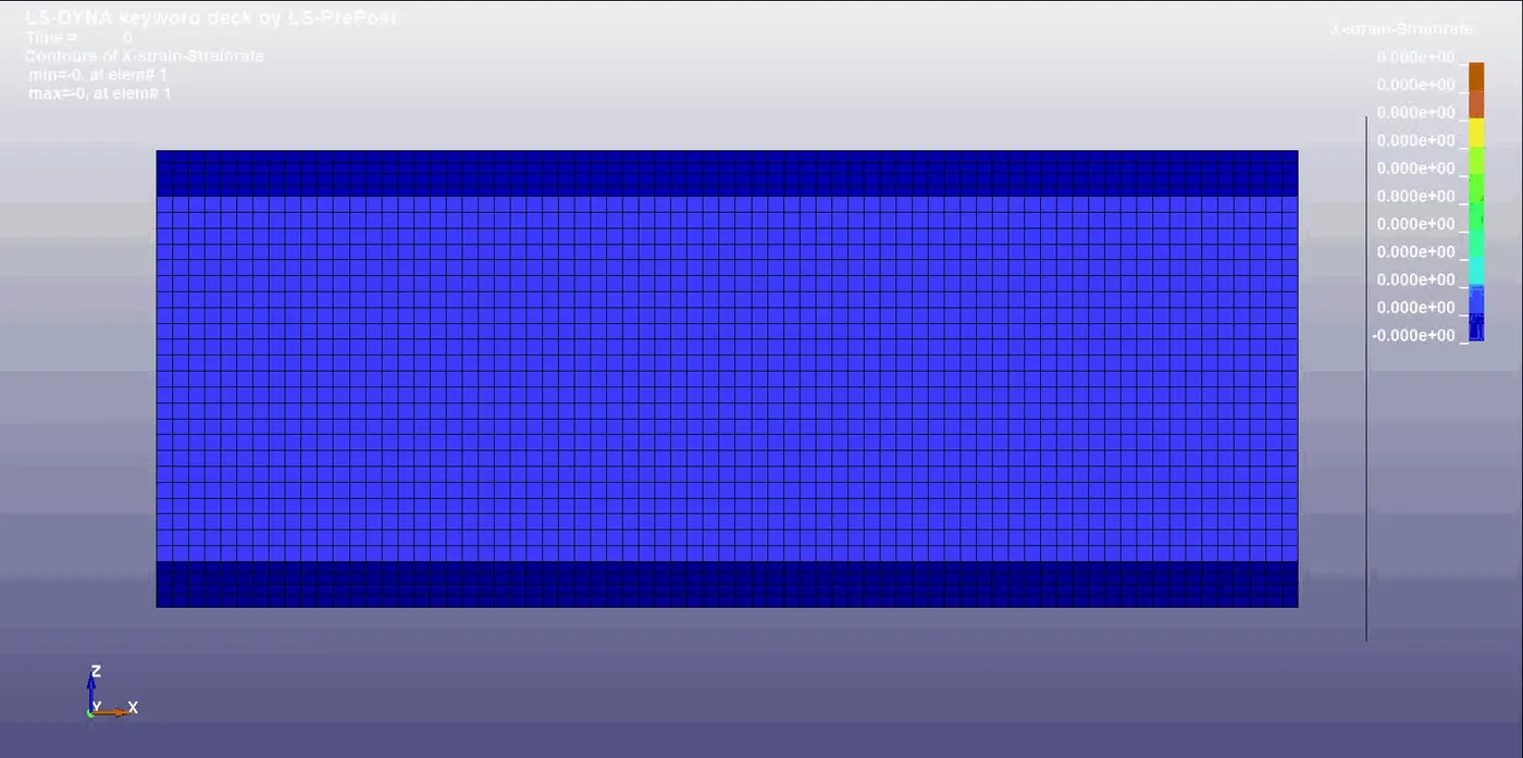
The min X directional Strain is found to be at -1.00813 at element no 4658 and the max X directional Strain is found to be 0.739579 at element 2303.

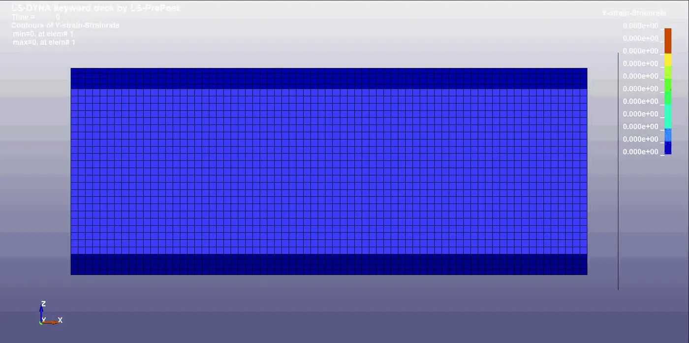
The min Y directional Strain is found to be at -0.112967 at element no 4664 and the max Y directional Strain is found to be 0.126947 at element 6062.

Plotting:

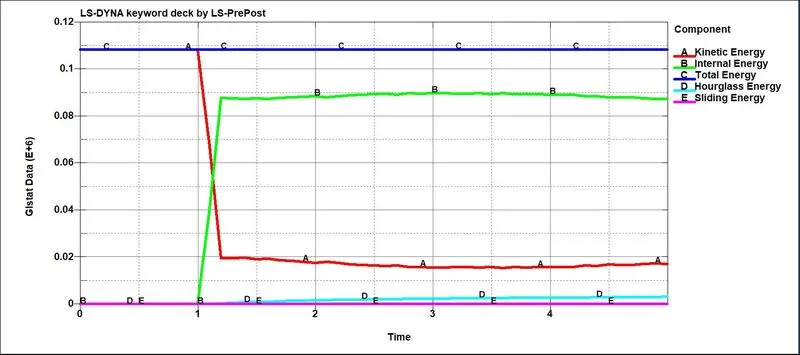
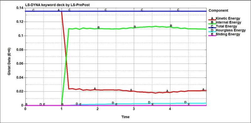
5) After we see the animation contours, we plot the energies, section forces, and nodal acceleration using the ASCII tab in the Post-processing tab. First, we plot the global data for both 1.2 and 1.5 mm Crash boxes i.e. the glstat which consists of internal energy, kinetic energy, hourglass energy, sliding energy, and total energy.

Crash box 1.2 mm:

Max Internal Energy: 9,000 J

Max Kinetic Energy: 11,000 J

Max Hourglass Energy: 3,000 J

Max Total Energy: 10,833.5 J

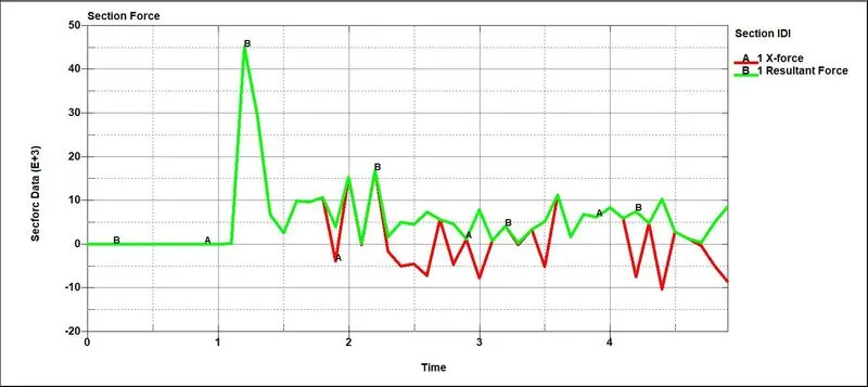
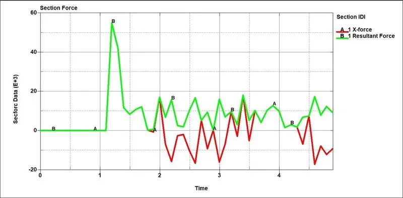
Peak Force During Impact: 4.5 KN

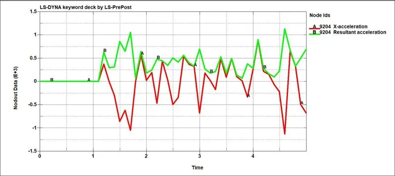
Peak acceleration during impact: 1.2 mm/ms^2

Crash box 1.5 mm:

Max Internal Energy: 11,300 J

Max Kinetic Energy: 13,500 J

Max Hourglass Energy: 3,200 J

Max Total Energy: 10,833.5 J

Peak Force During Impact: 5.5 KN

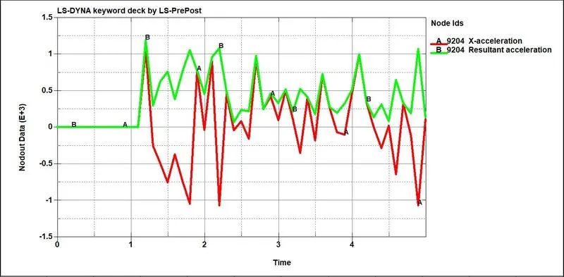
Peak acceleration during impact: 0.8 mm/ms^2

Comparison:

Global Energies:

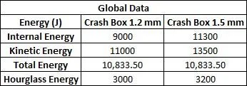
If we notice the internal energy of the crash box with 1.5mm Thickness which has more internal energy than a crash box with 1.2mm thickness which means the crash box with 1.5mm will absorb more energy than the crash box with 1.2mm. The hourglass energy in both cases is more than 15% so there are two ways to sort it out first one is to use a fully integrated formulation in shell properties and the other method is to use the hourglass control method.

Directional Stress and Strain:

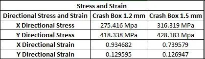
The X directional stress is more in the 1.5 mm Crash box because the initial velocity applied to it decreases the acceleration and has more stress.

Cross-sectional force and acceleration at node:

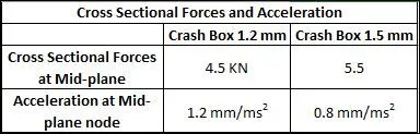
As we can see The Cross-section force for a Crash box with 1.5 mm thickness is more. This is because the Crash box with 1.5 mm thickness has extra mass compared to 1.2mm shell thickness with the same velocity values in both cases. So the extra mass is responsible for producing extra force values at the same velocity. It shows the peak acceleration is more in the crash box with 1.2 thickness and We can see the acceleration values for the X direction are negative. This is because the crash box is stopped by a rigid wall and thus deaccelerates. Whereas the resultant acceleration is the magnitude hence positive and almost equal to X-direction acceleration value because Y and Z direction accelerations being very small in comparison.

Conclusion:

1) We have initially set up the crash box models by assigning section, material, boundary conditions, control cards, and database.

2) We have the unit system to gm-mm-ms through the simulation.

3) We have also kept an initial velocity of 50kmph for the crash box.

4) We have simulated for both cases i.e. 1.2 mm Crash box and 1.5 mm Crash box.

5) We have plotted contour animations of Directional Stresses and Strains and also we have plotted the graphs for Global data, cross-sectional force at midplane, and acceleration at midplane node.

6) We can conclude that Crashbox with 1.5mm thickness is better than 1.2 mm thickness because the crash box with 1.5mm has more internal energy which absorbs more energy.