Curve Fitting for a Linear and Cubic Polynomial using Python

Aim:

1) Definition of popt and pcov in the curve fitting code in python.

2) Significance of np.array(temperature) in the curve fitting code in python.

3) Definition of * in *popt in the curve fitting code in python.

4) Writing a code to fit a linear and cubic polynomial for the given Cp data and explaining if the results are good or bad.

5) Procedure for obtaining perfect fit.

6) Empirically showing how well the curve has been fit.

Theory:

• CURVE FITTING:

Curve fitting is the process of constructing a curve, or mathematical function, that has the best fit to a series of data points, possibly subject to constraints. Curve fitting can involve either interpolation, where an exact fit to the data is required, or smoothing, in which a "smooth" function is constructed that approximately fits the data.

• POLYNOMIAL CURVE FITTING:

It is process of fitting the curve with the help of polynomial equations.

Generally linear, quadratic and cubic polynomials are taken for curve fitting.

1) Linear Polynomial: It is the polynomial equation of degree 1.

`y = a*x + b`

2) Quadratic Polynomial: It is the polynomial equation of degree 2.

`y = a*x^2 + b*x + c`

3) Cubic Polynomial: It is the polynomial equation of degree 3.

`y = a*x^3 + b*x^2 + c*x + d`

ERRORS IN CURVE FITTING:

Error=|y(i)-value of f(x) at x(i)|=|y(i)-f(x(i))|

To remove the modules sign we square the error term which Sum Square of Errors.

`S S E = sum_(i=0)^n ( Y ( i ) − f ( x ( i ) ) )^2`

We have to also find Sum of Squares of Regression.

`S S R = sum_(i=0)^n ( f ( x ( i ) ) − M e a n )^2`

After finding the SSE and SSR we have to find the SST which basically of both SSE and SSR.

`S S T=S S R+S S E`

After that R square is calculated from the following formula.

`R^2 = (S S R)/(S S T)`

After we find Root Mean Square Error(RMSE) which is known Standard fit error.

`R M S E = sqrt((sum_(i = 1)^n ( Y ( i ) − f ( x ( i ) ) )^2)/n) = sqrt((SSE)/n)`

Procedure:

1. Definition of popt and pcov in the curve fitting code in python.

Popt is an array returned by the curve fit function that contains the optimised value of the parameters of the function passed to curve_fit. In this case, it is an array containing the optimum values of the coefficients of the function in order to obtain the plot that best fits the given data.

Pcov is a matrix whose diagonal elements contain the variance of popt which can be extracted and its square root provides the standard deviation for error from the original data points.

2. Significance of np.array(temperature) in the curve fitting code in python.

It is an operation possible through numpy module which passes the array containing the range of temperature to the desired function or operation.

3. Definition of * in *popt in the curve fitting code in python.

The * here is used to refer to the values generated and stored in the popt array in order to obtain the curve fit.

4 & 6. Writing a code to fit a linear and cubic polynomial for the given Cp data. Empirically showing how well the curve has been fit.

• Full Code:

#Curve Fitting Challenge

#Importing all the Libraries

import math
import matplotlib.pyplot as plt 
import numpy as np 
from scipy.optimize import curve_fit

#Defining a function for solving in linear polynomial 

def f_order1(t,a,b):

	a*t + b
	return a*t + b

#Defining a function for solving in cubic polynomial 

def f_order3(t,a,b,c,d):

	a*pow(t,3) + b*pow(t,2) + c*t + d
	return a*pow(t,3) + b*pow(t,2) + c*t + d

#reading data from the file, named 'data'

def read_file():
	
	temperature = []
	cp = []
	for line in open ('data','r'): # reading each line of file
		line=line.split(',')
		temperature.append(float(line[0])) # storing the values of temperature in temperature array
		cp.append(float(line[1]))  # storing the values of cp in array cp
		
	return [temperature, cp]

# Optimizing the curve for linear polynomial

temperature, cp = read_file()
popt_1, pcov_1 = curve_fit(f_order1, temperature, cp)
new_cp_1 = f_order1(np.array(temperature), *popt_1)

#Calculating goodness of linear fit

#SSE
sse = 0
for i in range(0,np.size(cp)):
	sse = sse + pow(cp[i]-new_cp_1[i],2)

print('For linear polynomial fit,')

#R_square 
mean =np.sum(cp)/np.size(cp)
ssr=0
for i in range(0,np.size(cp)):
	ssr = ssr + pow(new_cp_1[i] - mean,2)

sst = ssr + sse 
R_square = ssr/sst
print('R_square = ',R_square)

#RMSE
rmse=pow(sse/np.size(cp),0.5)
print('RMSE = ',rmse)

# Optimizing the curve for cubic polynomial

temperature, cp = read_file()
popt_3, pcov_3 = curve_fit(f_order3, temperature, cp)
new_cp_3 = f_order3(np.array(temperature), *popt_3)

#Calculating goodness of cubic polynomial fit

#SSE
sse = 0
for i in range(0,np.size(cp)):
	sse = sse + pow(cp[i]-new_cp_3[i],2)

print('For cubic polynomial fit,')

#R_square 
mean =np.sum(cp)/np.size(cp)
ssr=0
for i in range(0,np.size(cp)):
	ssr = ssr + pow(new_cp_3[i] - mean,2)

sst = ssr + sse 
R_square = ssr/sst
print('R_square = ',R_square)

#RMSE
rmse=pow(sse/np.size(cp),0.5)
print('RMSE = ',rmse)

#Plotting for linear polynomial curve fit

plt.figure(1)
plt.plot(temperature, cp, linewidth=3, color='blue')
plt.plot(temperature, new_cp_1, linewidth=3, color='red')
plt.legend(['actual data', 'curve fit'])
plt.xlabel('Temperature[K]')
plt.ylabel('cp')
plt.grid()
plt.title('Linear polynomial curve fit')
plt.savefig('Linear polynomial curve fit.png')
plt.show()

#Plotting for cubic polynomial curve fit

plt.figure(2)
plt.plot(temperature, cp, linewidth=3, color='blue')
plt.plot(temperature, new_cp_3, linewidth=3, color='red')
plt.legend(['actual data', 'curve fit'])
plt.xlabel('Temperature[K]')
plt.ylabel('cp')
plt.grid()
plt.title('Cubic polynomial curve fit')
plt.savefig('Cubic polynomial curve fit.png')
plt.show()

1) We first import all the libraries like math, matplotlib.pyplot, numpy & scipy(for curve fitting).

2) We then, define the function for linear polynomial and cubic polynomial.

3) We define another function for reading the data file in the for loop so that we can read both temperature and Cp data's and we use float command to take the numbers after decimal point in the data file.

4) We use the popt and pcov commands to return an array by the curve fit function and to get square root provides the standard deviation for error from the original data points.

5) We then calculate the SSE, SSR, SST, R square and RMSE and print it.

6) Then, we plot the graphs for Linear and Cubic Fit with the Actual Data.

7) After that we save the figure plotted.

5. Procedure for obtaining perfect fit.

A perfect fit is the one which completely fits the data without any errors. Now, there could be several ways to obtain a perfect fit like using a higher degree polynomial. However, it is not always guaranteed that increasing the degree of the polynomial would give a perfect fit. Therefore, other methods like using the split-wise polynomial is used. In this, the range is divided into several sub-ranges and a polynomial of a suitable degree is assigned to each range in order to improve the goodness of fit. There is another way to obtain a perfect fit and that is by centering and scaling.

Results and Discussion:

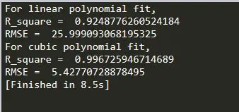
The results obtained for the linear polynomial fit is a good fit since Rsquare value is 0.9248 and for the cubic polynomial fit the result is best fit since the Rsquare value is 0.9967 which is almost a perfect fit. There results window screenshot after calculating the SSE, SSR, SST, R square and RMSE for linear and cubic fit are given in the image given below.

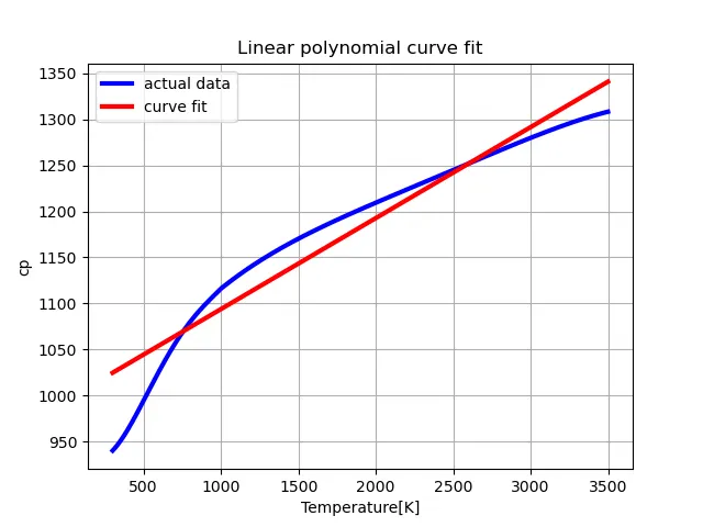
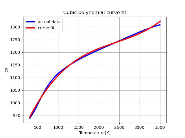
The graphs are also plotted for the linear and cubic polynomial with actual data. The images given below shows that cubic polynomial curve fit is better than linear polynomial curve fit as it almost follows the path of the actual data curve.

Conclusion:

1) We have the defined the popt and pcov in the curve fitting code in python.

2) We have defined the significance of np.array(temperature) in the curve fitting code in python.

3) We have Defined the significance of * in *popt in the curve fitting code in python.

4) We have written a code to fit a linear and cubic polynomial for the given Cp data and explained if the results were good or bad.

5) We have also written the procedure for obtaining perfect fit.

6) We have empirically shown in the coding itself how well the curve has been fit.