Solving and Simulating Second Order ODE's for Simple Pendulum using Python
Objective:
1) To simulate the transient behaviour of a simple pendulum using second order ODE's using python.
2) To plot displacement and velocity graph.
3) To create an animation of pendulum motion.
Theory:
- ORDINARY DIFFERENTIAL EQUATION:
An ordinary differential equation (ODE) is a differential equation containing one or more functions of one independent variable and the derivatives of those functions.
- Second Order ODE's:
An ODE with the form y''+P(x)⋅y'+Q(x)⋅y=0y′′+P(x)⋅y′+Q(x)⋅y=0is known as Second Order ODE's.
- SIMPLE PENDULUM:
A simple pendulum consists of a mass m hanging from a string of length L and fixed at a pivot point P. When displaced to an initial angle and released, the pendulum will swing back and forth with periodic motion. By applying Newton's secont law for rotational systems, the equation of motion for the pendulum may be obtained.
The Second order ODE for a Simple Pendulum with damping is
`( (d^2 θ)/(d t^2) ) + ( b/m ) * ( (dθ)/(dt) ) + ( g/l )*sin(theta) = 0`
Here, b= damping coefficient
m= mass of the ball hanging (kg)
l= length of the string (m)
g= acceleration due to gravity (m/sec^2)
θ= Angle made by the string with attached during transient motion (degrees)
Procedure:
- Full Code:
import math
import matplotlib.pyplot as plt
import numpy as np
from scipy.integrate import odeint

# Defining a Function
def model(theta,t,b,g,l,m):
	theta1=theta[0]
	theta2=theta[1]
	dtheta1_dt=theta2
	dtheta2_dt= -(b/m)*theta2 - (g/l)*math.sin(theta1)
	dtheta_dt=[dtheta1_dt,dtheta2_dt]
	return dtheta_dt

# Inputs
b=.05   #Damping Coefficient
g=9.81  #Acceleration due to gravity (in m/s^2)
l=1     #length of pendulum(in metre)
m=1     #mass of ball(in kg)

# Initial condition
theta_0=[0,3]         #First value is angular displacement and second value is angular velocity

# Time inputs
t=np.linspace(0,20,200)    #time is defined bw 0 to 20sec and there are 200 points in between

#Solving the ODE
theta=odeint(model,theta_0,t,args = (b,g,l,m))

#Plotting
plt.figure()
plt.plot(t,theta[:,0],'b-',label='Displacement')
plt.plot(t,theta[:,1],'r--',label='Velocity')
plt.legend()
plt.xlabel('Time')
plt.ylabel('Plot')
plt.xlim([0,20])
plt.grid('on')
plt.savefig('Plot')
plt.show()


#Creating an animation
ct=1
for theta in theta[:,0]: #Animation is made with the help of positions obtained in solution

	x0=0
	y0=0
	x1=l*math.sin(theta)
	y1=-l*math.cos(theta)
	filename=str(ct)+'.png'
	plt.figure()
	plt.plot([-1.5,1.5],[0,0],"red",linewidth=5)
	plt.plot([x0,x1],[y0,y1],"blue")
	plt.plot(x1,y1,'o',color="green",markersize=10)
	plt.xlim([-1.5,1.5])
	plt.ylim([-1.5,1.5])
	plt.savefig(filename)
ct=ct+1- Step wise Explanation:
1) We first import the math, plotting,numpy and scipy liibrares. The scipy library is used to solve ordinary differential equation and we import odeint library from it.
2) We define a function and we input all the ODE's into it.
If theta is considered as θ=θ1 then
`(dθ)/(dt) = (dθ_1)/(dt) = θ_2`
`(d^2θ)/(dt^2) = (d^2θ_1)/(dt^2) = (d)/(dt) ⋅ ( dθ_1)/(dt) = (d)/(dt)*θ_2`
The above second order equation of simple pendulum becomes
`(dθ_2)/(dt) + (b/m)* θ_2 + (g/l)*sin θ_1 = 0`
`(dθ_2)/(dt) = − (b/m)*θ_2−(g/l)*sin θ_1`
3) Initial inputs namely Damping Coefficient (b), Mass (m), Acceleration due to gravity (g) & length of the string (l) are provided.
4) The intial conditions of Angular Displacement and Angular Velocity are given under variable theta_0. After that the time intervals are also provided using the linspace command which prints the Angular Displacement and Angular Velocity how much ever times required.
5) We use odeint to solve the ODE's given to us and we finally use the plotting command to plot the graph between time and plot to plot different values of displacement and velocity.
6) We then proceed for creating animation for that we first assign a counter variable ct.
7) We then perform maths operation to plot the simple pendulum base, the string and the hanging pendulum ball.
8) We plot the graph and assign x limits and y limits so that the animation seen in the middle of the plotting area.
9) We run the program using the CTRL+B and get the plot for time vs plot and 200 images for different positions of the pendulum.
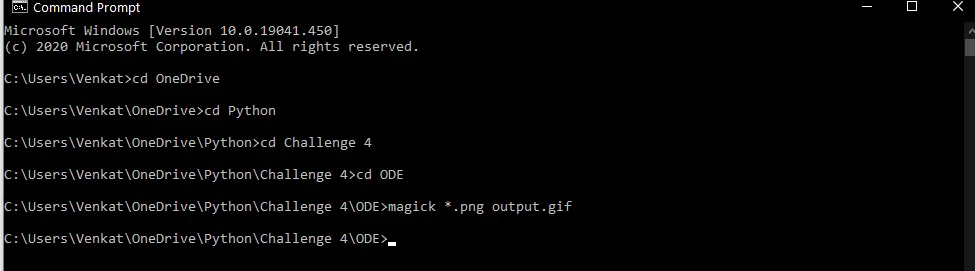
10) We need to stitch those images to form a animation or gif file for we use the image magick application. We get the output using the command prompt as shown in the image given below.
Results and Discussion:
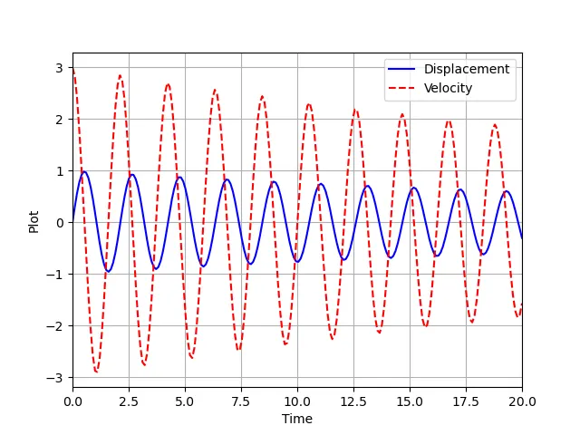
1) On running the program we get the time vs plot graph which shows different values of angular displacement and angular velocity in form of sin and cos waves as shown in the image given below.
2) We also get the animation of the pendulum motion in the gif format we change it to video format.
Animation:
The animation link is given below.