Analysis and Comparison of 2D shell elements in a Crash tube with and without the recommended shell formulations in Radioss

Aim:

The main aim of Assignment-3 is to make a comparison of results with base simulation and improved shell element properties,and To perform the various challenges which are listed below.

1.Using the crash beam file from the previous assignment, change the run time to 55 ms.

2. Change the number of animation steps during simulation to a minimum of 25 and maximum of 60.

3. Run the base simulation without any modification to element properties.

4. At the end of the simulation, do the energy error and mass error checks and determine whether results would be acceptable.

5. If acceptable, Plot rigid wall forces, internal energy, hourglass energy, contact energy, total energy of the simulations.

6. Change all the shell elements properties to recommended properties, save this as separate, rad files and run the simulation.

7. Follow steps 5 and 6.

8. Create a brief report comparing all the results from steps 5 and 6 for both simulations.

9. Comment whether there is any change in the results and why there is any change in the result.

The reccomended shell element properties for quesion 6 are also given below.

Parameters		Comment
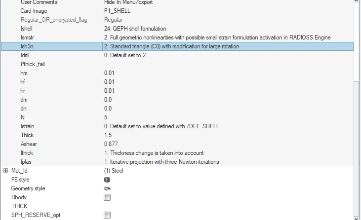
Ishell =24		QEPH 4 nodes shells are best combination of cost and accuracy.
Ismstr=2		Full geometric nonlinearities (default)with possible small strain formulation activation in RADIOSS Engine.
Ish3n=2		Standard 3 noded shell (C0)with modification for large rotation(default)
N=5		Number of integration points set to 5 for accuracy bending.
Ithick=1		Thickness change is taken into account for accuracy.
Iplas=1		Iterative plasticity for good accuracy.

Procedure:

1. Using the crash beam file from the previous assignment, change the run time to 55 ms.

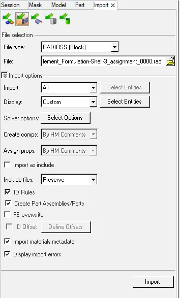
1) We first import the crash beam file from the previous assignment by using import solver deck option as shown in the image given below.

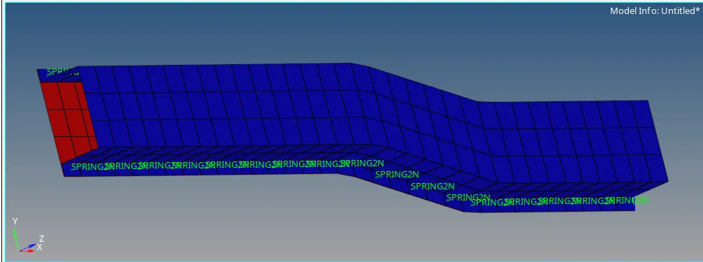
2) The imported model is in wireframe mode therefore, we have to change it to the shaded mode using the Shaded Elements and Mesh Lines option as shown in the image given below.

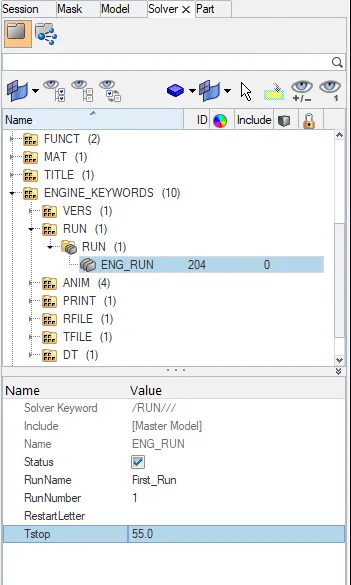
3) We then go to the Solver Browser option and click on the Engine Keywords option and under we click on the Run option to view the termination time. We click on the ENG_RUN option and in the Editor Window we input the value of Tstop as 55 ms instead of 60 ms as shown in the image given below.

2. Change the number of animation steps during simulation to a minimum of 25 and maximum of 60.

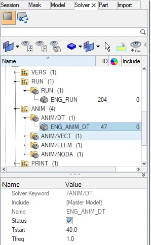
4) We then, go to the Solver Browser option again and click on the ANIM/DT option and then, under it we click on the ENG_ANIM_DT option and in the Editor Window we input the value of Tstart as 40 since the values can be between 25 to 60.

We input this value in the Editor Window as shown in the image given below.

3. Run the base simulation without any modification to element properties.

5) We don't modify any element properties and keep it as default for all the parts of the model as shown in the images given below.

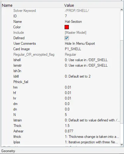
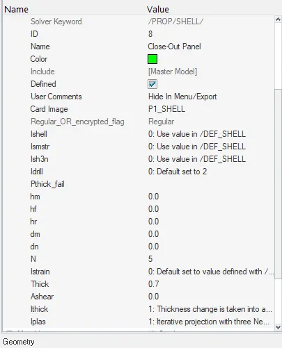
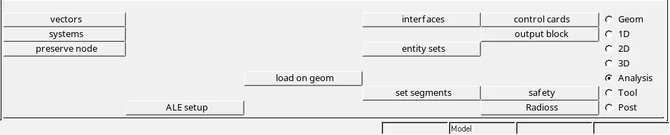
6) We have to run the simulation the using default values of element properties for that, we go to the Analysis module and click on Radioss option under it as shown in the image given below.

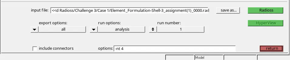
7) We get a new window to save the input file, we review on it and then we press Saveas button, Then we, give the export options as all, the run options as analysis and the run number as 1. We, then mention the options as -nt 4 as we need our simulation to get it done faster and then, finally we click on Radioss to run the simulation. The window is shown in the image given below.

4. At the end of the simulation, do the energy error and mass error checks and determine whether results would be acceptable.

8) We run the simulation and we get the simulation result. Then we go to the folder were the output file has been saved. We open the output file 'Element_Formulation-Shell-3_assignment(1)_0001.out' in the the text editor format to findout the Energy error and Mass error as shown in the image given below.

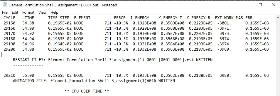
9) In the above image we find that the maximum energy error and mass error at the end of the simulation are -10.3 % and 0.1659E-03. Basically energy error must be between -15% to 5% at the end of computation, as per the condition. If the error is below negative than the results could be acceptable. As per the condition the energy error is -10.3% which is acceptable and we can move for plotting the graphs.

5. If acceptable, Plot rigid wall forces, internal energy, hourglass energy, contact energy, total energy of the simulations.

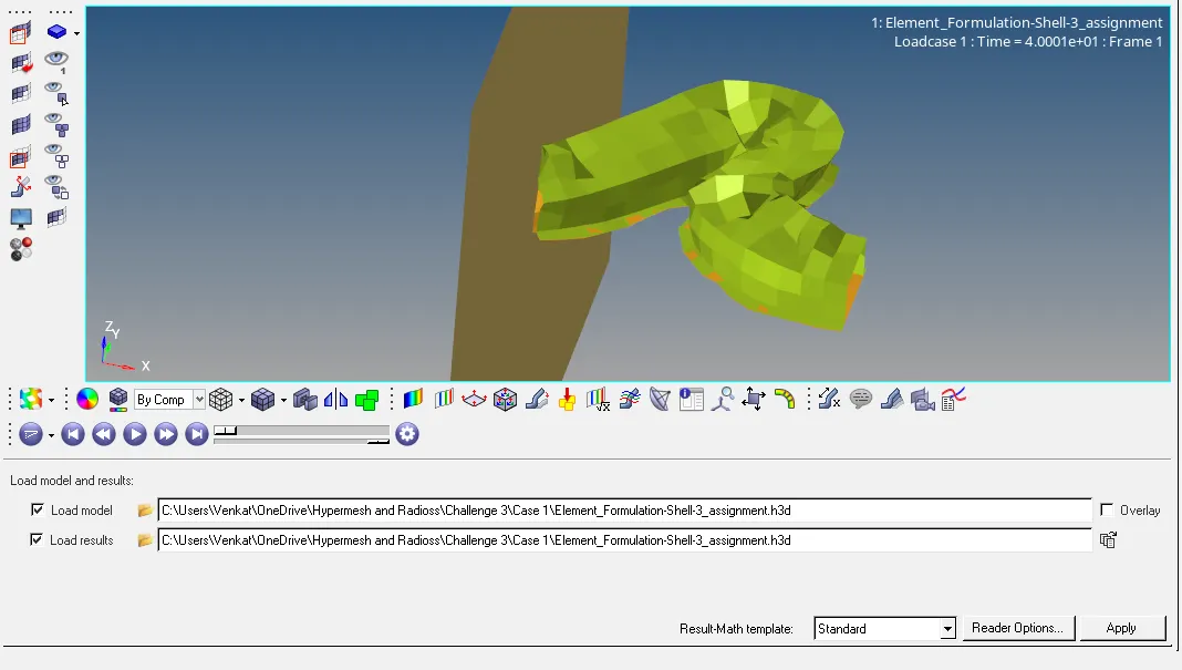
10) After finding out the energy error and mass error we go to the Hyperview and import the 'Element_Formulation-Shell-3_assignment.h3d' file and we can see the rigid wall and deformed beam loaded together. We see that the beam is deformed since we have given animation steps during simulation as 40ms, therefore it has started capturing animation frames after 40ms till 55ms i.e. the end. The deformed beam is shown in the image given below.

11) The Various plots of the deformed beam are obtained. These consist of both 2D plots using Hypergraph 2D and contour plots using Hyperview. The different plots are given below.

1. Displacement Contour Plot:

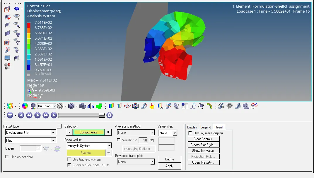
For displacement contour plot we first click on the Contour option present in the HV Result tab and under it we select the result type as Displacement and then we the select component and give apply option. We get the Min value= 9.759E-03 and Max value = 7.611E+02 as shown in the image given below.

2. Von Misses Contour Plot:

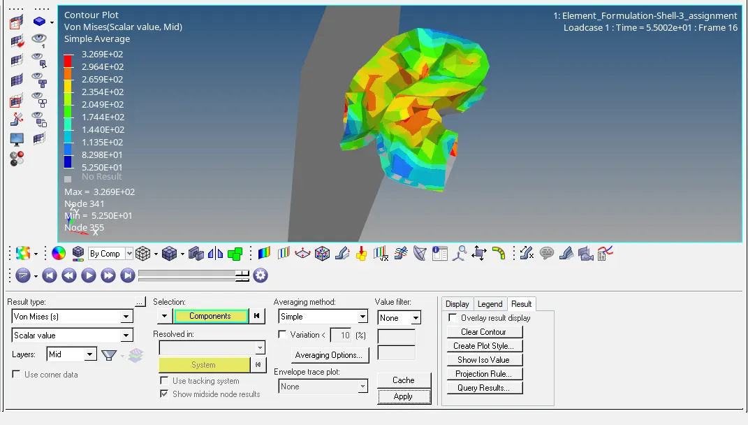
For von misses contour plot we first click on the Contour option present in the HV Result tab and under it we select the result type as Von Misses , we also select averaging type in this as Simple and then we the select component and give apply option. We get the Min value= 5250E+01 and Max value = 3.269E+02 as shown in the image given below.

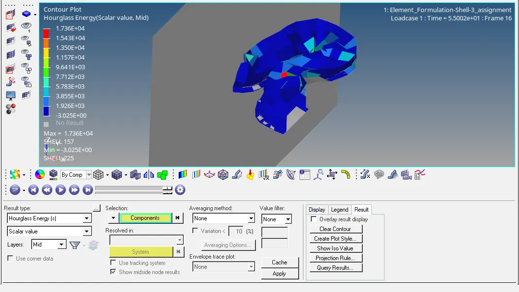
3. Hourglass Contour Plot:

For hourglass contour plot we first click on the Contour option present in the HV Result tab and under it we select the result type as Hourglass Energy and then we the select component and give apply option. We get the Min value= -3.025E+00 and Max value = 1.736E+04 as shown in the image given below.

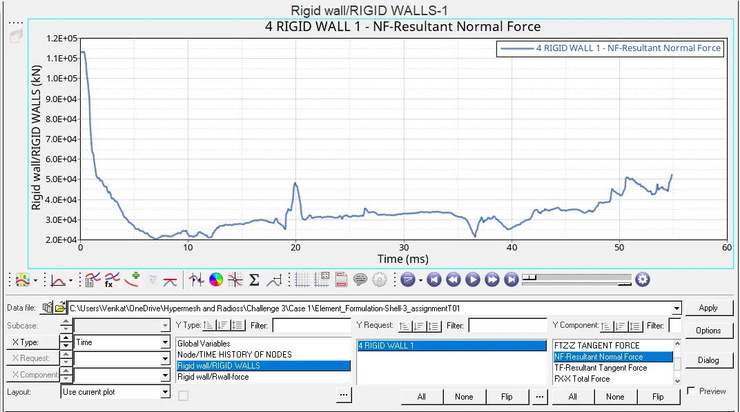
4. Rigid Wall Forces 2D Plot:

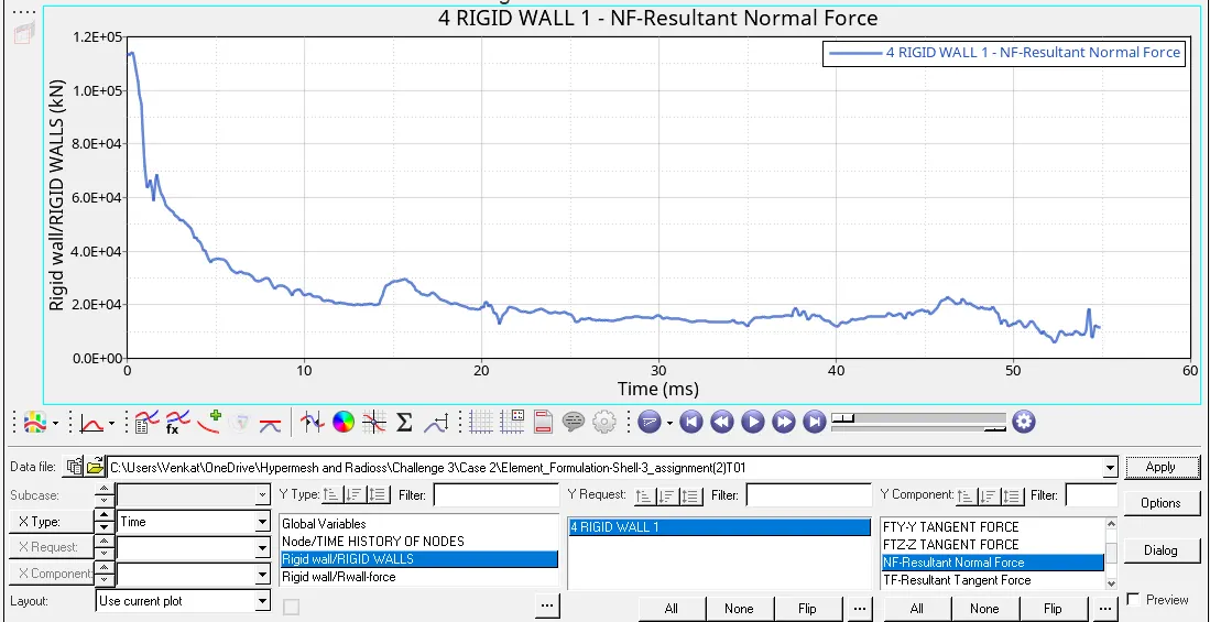
For rigid wall forces plot we first click on the Hypergraph 2D option and under it we import the 'Element_Formulation-Shell-3_assignmentT01' file. We then click on X-type value as Time and Y-type value as Rigid wall, Y-Request as 4 Rigid Wall 1 & Y-Component as NF- Normal Resultant Force. Then we give apply and the rigid wall force shows a Maximum force of 1.14E+05 KN. The graph is shown in the image given below.

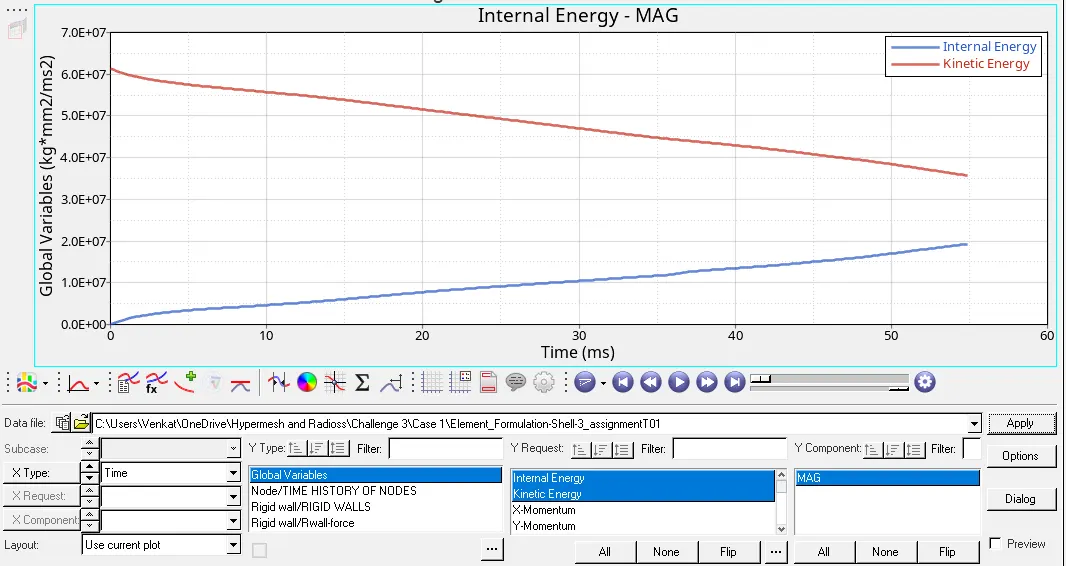
5. Internal Energy and Kinetic Energy 2D Plot:

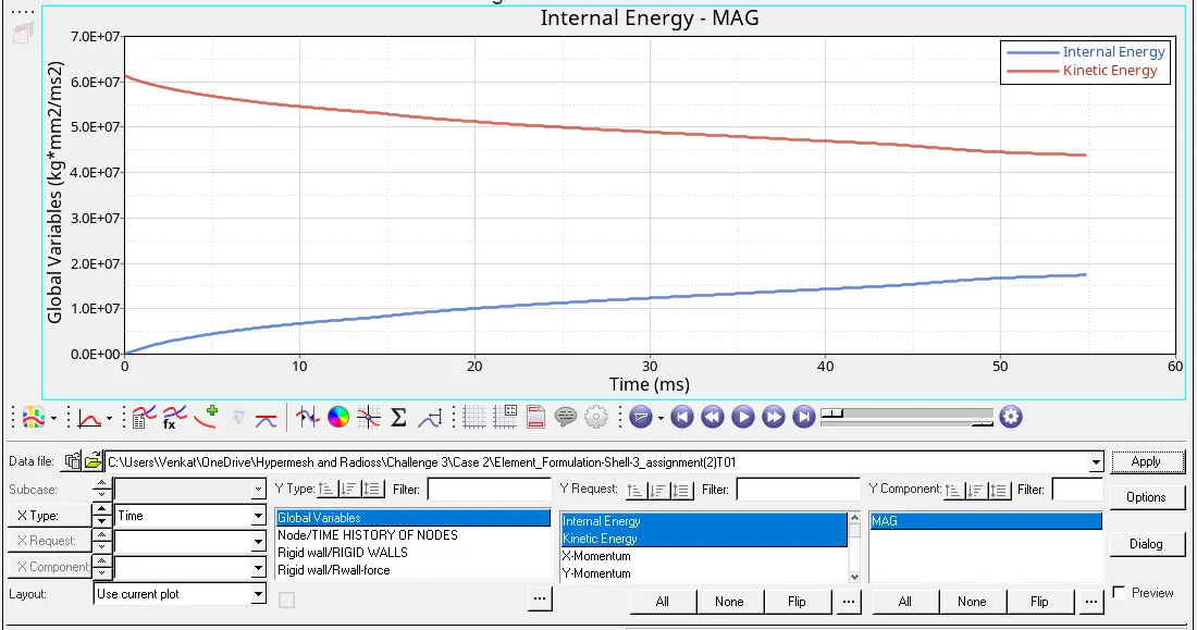
For internal and kinetic energy plot we first click on the Hypergraph 2D option and under it we import the 'Element_Formulation-Shell-3_assignmentT01' file. We then click on X-type value as Time and Y-type value as Global Variables, Y-Request as Internal Energy/Kinetic Energy & Y-Component as MAG. From the graph the internal energy slowly increases from Minimum value of 0.0E+00 to a maximum value of 2.0E+07 and the kinetic energy slowly decreases from Maximum value of 6.1E+07 to a Minimum value of 3.5E+07.The graph is shown in the image given below.

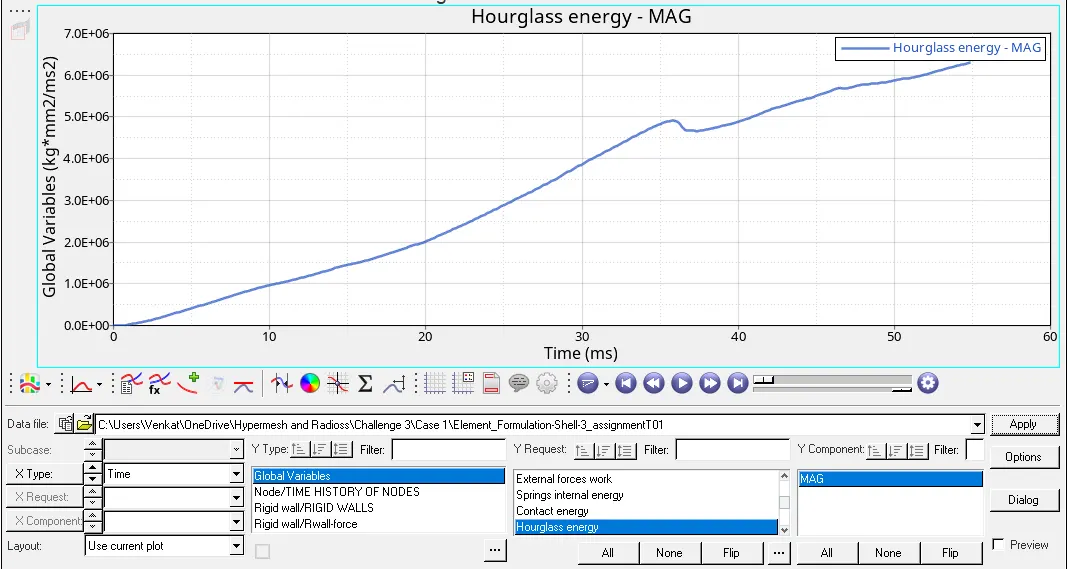
5. Hourglass Energy 2D Plot:

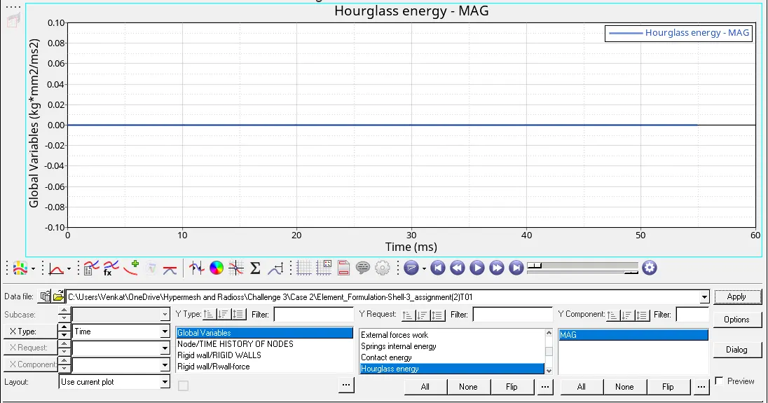
For hour glass energy plot we first click on the Hypergraph 2D option and under it we import the 'Element_Formulation-Shell-3_assignmentT01' file. We then click on X-type value as Time and Y-type value as Global Variables, Y-Request as Hour Glass Energy & Y-Component as MAG. The graph is shown in the image given below.

6. Contact Energy 2D Plot:

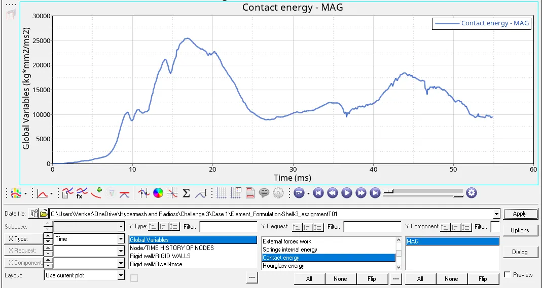
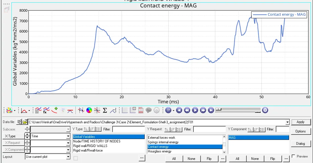
For contact energy plot we first click on the Hypergraph 2D option and under it we import the 'Element_Formulation-Shell-3_assignmentT01' file. We then click on X-type value as Time and Y-type value as Global Variables, Y-Request as Contact Energy & Y-Component as MAG. The graph is shown in the image given below.

7. Total Energy 2D Plot:

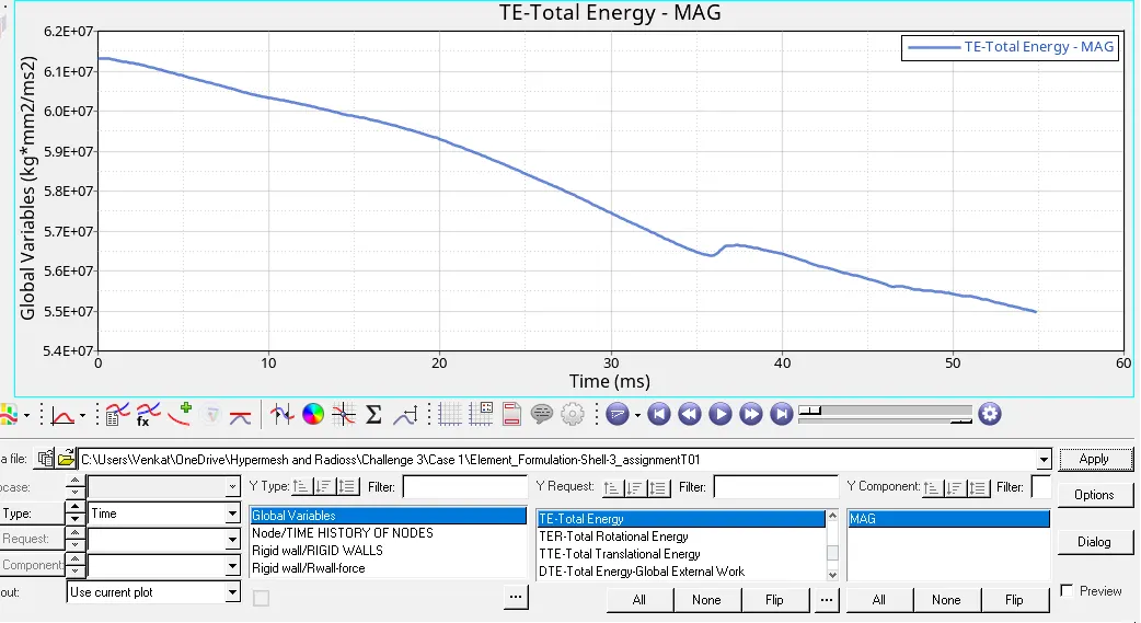
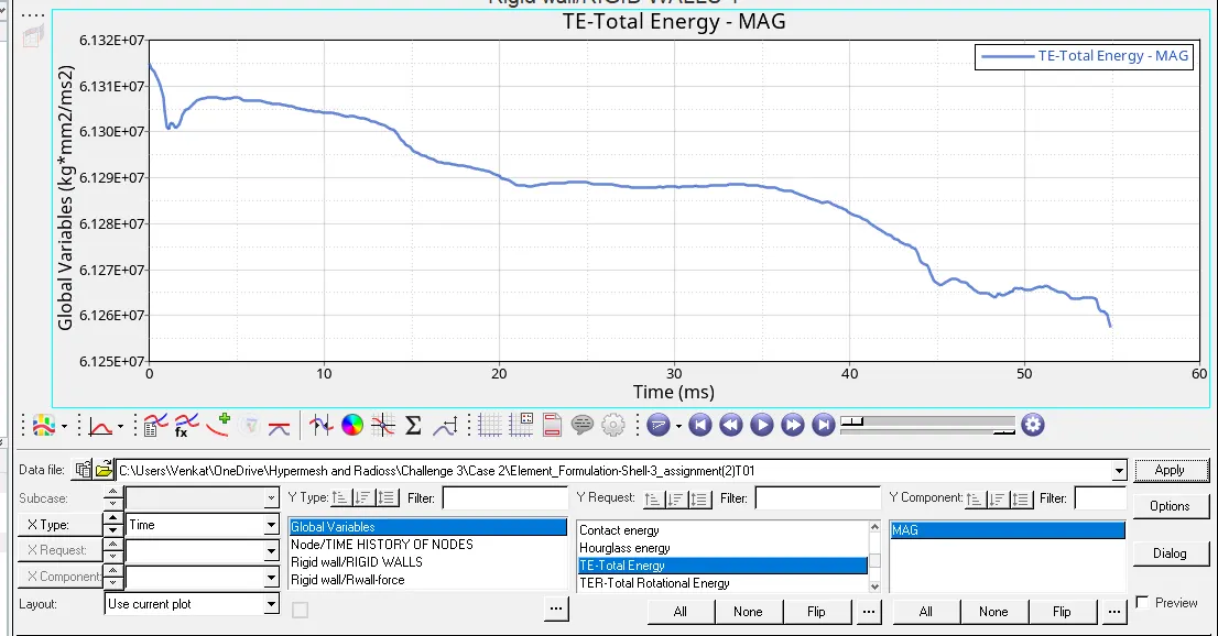
For total energy plot we first click on the Hypergraph 2D option and under it we import the 'Element_Formulation-Shell-3_assignmentT01' file. We then click on X-type value as Time and Y-type value as Global Variables, Y-Request as Total Energy & Y-Component as MAG. The graph is shown in the image given below.

6 & 7. Change all the shell elements properties to recommended properties, save this as separate, rad files and run the simulation. Follow steps 5 and 6.

1) We modify the element properties according to the parameters given in the aim and change it for all the parts of the model as shown in the image given below.

2) We then run the simulation the using default values of element properties for that, we go to the Analysis module and click on Radioss option under it. We get a new window to save the input file, we review on it and then we press Saveas button, Then we, give the export options as all, the run options as analysis and the run number as 1. We, then mention the options as -nt 4 as we need our simulation to get it done faster and then, finally we click on Radioss to run the simulation as shown.

3) We run the simulation and we get the simulation result. Then we go to the folder were the output file has been saved. We open the output file 'Element_Formulation-Shell-3_assignment(2)_0001.out' in the the text editor format to findout the Energy error and Mass error as shown in the image given below.

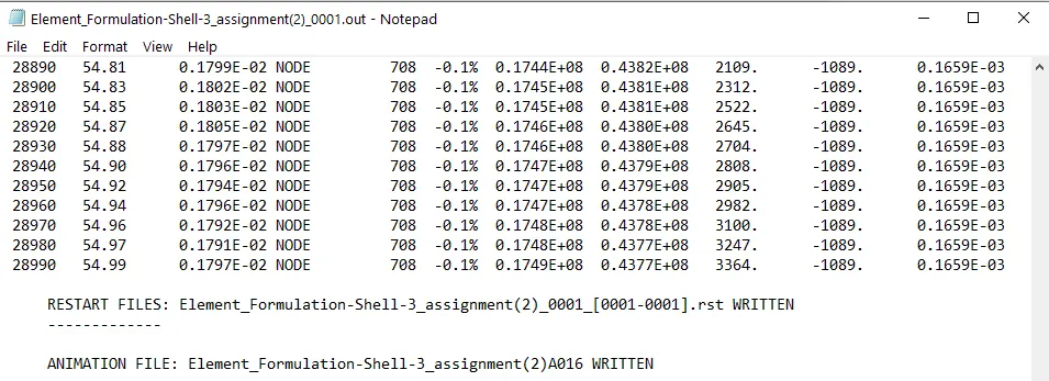
4) In the above image we find that the maximum energy error and mass error at the end of the simulation are -0.1 % and 0.1659E-03. Basically energy error must be between -15% to 5% at the end of computation, as per the condition. If the error is below negative than the results could be acceptable. As per the condition the energy error is -0.1% which is acceptable and we can move for plotting the graphs.

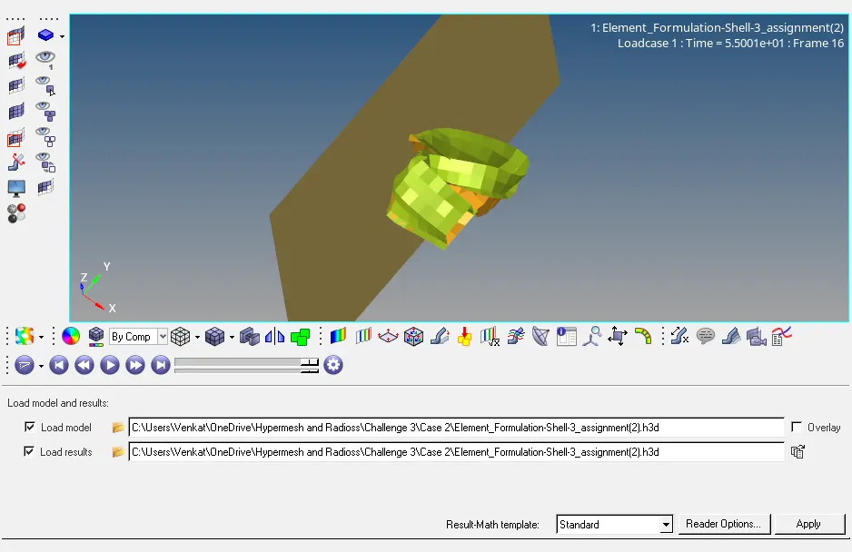
5) After finding out the energy error and mass error we go to the Hyperview and import the 'Element_Formulation-Shell-3_assignment(2).h3d' file and we can see the rigid wall and deformed beam loaded together. We see that the beam is deformed since we have given animation steps during simulation as 40ms, therefore it has started capturing animation frames after 40ms till 55ms i.e. the end. The deformed beam is shown in the image given below.

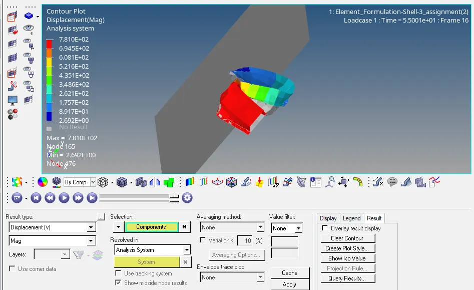
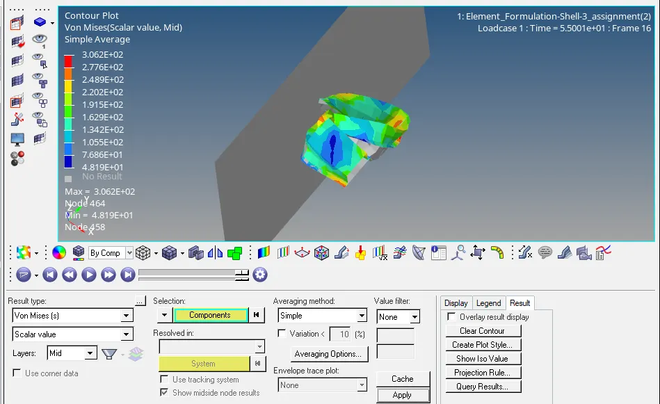
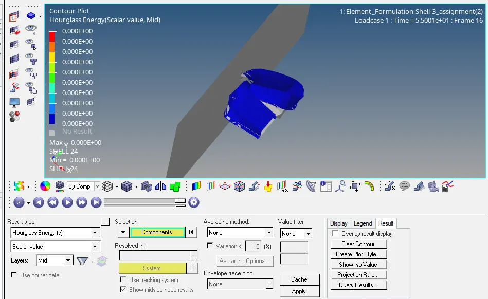
6) We follow the same process for plotting the contour plots and we get the contour plots for Displacement, Von Misses and Hour glass energy using the Contour option in the HV Result tab. The contour plots are shown in the images given below.

7) We also follow the same process for plotting the 2D plots and we get the 2D plots for Rigid Wall Forces, Internal & Kinetic Energy, Hourglass Energy, Contact Energy and Total energy using the Hypergraph 2D option. The 2D plots are shown in the images given below.

Results and Discussion:

8 & 9. Create a brief report comparing all the results from steps 5 and 6 for both simulations. Comment whether there is any change in the results and why there is any change in the result.

Comparison Between Default Case and Element Formulation Case for Crash Beam Simulation
S.No	Parameters	Case-1	Case-2
1	Displacement Contour Plot	In this case the displacement is uneven because of the default shell properties are followed. The Min and Max Displacement values are 9.759E-03 and 7.611E+02	In this case the displacement is even because we have used the Qeph shell properties. The Min and Max Displacement values are 2.692E+00 and 7.810E+02
2	Von Mises Stress Contour Plot	In this case the von mises stress values are little higher because of the default shell properties are followed. The Min and Max Displacement values are 5.250E+01 and 3.269E+02	In this case the von mises stress values are on the lower side because of the Qeph shell properties are followed. The Min and Max Displacement values are 4.819E+01 and 3.062E+02
3	Rigid Wall Forces 2D Plot	In this case the rigid wall forces remain high(1.14E+05 KN) at the starting as the crash beam is colliding with the wall and finally decreases(1.6E+04 KN) at the end of the simulation.	In this case the rigid wall forces remain the same as the default one because the process is happening again.
4	Internal and Kinetic Energy 2D Plot	In this case the Kinetic Energy decreases(6E+07 to 3.5E+07) with time because there is no energy being stored in the system and the internal energy keeps on increasing(0 to 2E+07) with time because the straining of the material increases.	In this case the Kinetic Energy does have less effect because of the Qeph formulation, it decreases(6E+07 to 4.5E+07) with time because there is no energy being stored in the system and the internal energy has also less effect that keeps on increasing(0 to 1.8E+07) with time because the straining of the material increases.
5	Hour glass energy Contour and 2D Plot	In the default case the hourglass energy keeps on increasing(0 to 6.5 E+06) w.r.t time because we don't use any element formulations.	In the modified case the hourglass energy remains zero throughout the simulation because of the Qeph formulation we have used. This also shows that there is no artifical energies acting upon the crash beam.
6	Contact Energy 2D Plot	In the default case the contact energy keeps on increasing (0 to 26,000 J) since there so much contact between the shell elements and after that it decreases (10,000 J)	In the modified case the contact energy keeps on increasing (0 to 6,500 J) but the increase is not as high the previous case as the Qeph formulation is considered and finally it again increase to 7,500 J max because of element contact.
7	Total Energy 2D Plot	In the default case the total energy is calculated as sum of KE+IE+CE+HE and the total energy decreases (6.11E+07 to 5.6E+07) with the increase in time as the mass applied gets reduced at the end of the simulation.	In the modified case the total energy is calculated in the same way as the first case, it decreases (6.135E+07 to 6.125E+07) which less decreses than the initial case because of the Qeph formulation.

Hourglass Energy and its modes:

Hourglass modes are nonphysical mode of deformation that occurs in under integrated elements and produce no stress. Reduced integration can lead to non-physical zero-energy modes, called hourglass modes. There are two methods used to control the formulation of hour glassing:

Perturbation (Q4 Elements) ->Viscous method- damping is applied -> Due to damping deformation is stabilized -> that tries to control the velocities only ->Hour glass is an artificial energy. This method is used for very high-velocity problems such as explosive or bullet fire (100-1000m/s)

Physical Stabilization (QEPH Elements) -> Stiffness method -> Stiffness is added to material level so it may consistent. -> most of the time this method is preferred for analysis purpose. We have used this method in our analysis and we can see that the hourglass energy reaches zero which is an optimal result.

Conclusion:

1) There are two different types of radioss files namely engine file (runname_0001.rad) and starter file (runname_0000.rad).

2) We have learnt about how to change the run time during simulations using various types of radioss files.

3) We also have seen how the use of different shell properties and its use. Creation of property cards of different shell elements.

4) We can use different shell element formulation methods based on integration quality and relative cost. Based on this we can choose QEPH elements for Improved under Integration. This method gives physical stabilization for hourglass energy control.

5) When we choose shell element formulation as QEPH element the hourglass energy remains close to zero whereas when we are not using initial properties the hourglass energy increases drastically which will lead to a considerable % energy error.

6) The result reliability is strongly affected by the energy error percentage; if the error is negative it means some energy has been dissipated while it positive there is energy.

7) QEPH cell formation for fully integrated elements the energy error can be slightly positive since there is no hourglass energy and the computation is much more accurate.

8) An error of one or two percent will be acceptable otherwise any positive energy error means energy has been created which indicates a model issue.

Model Link:

https://drive.google.com/file/d/1k_khuRvdxBPNCN4b1BVdH02plvOelC4G/view?usp=sharing