Air Standard Cycle or Otto Cycle using Python

OBJECTIVE:

1) To simulate the Air Standard Cycle or the Otto Cycle using Python.

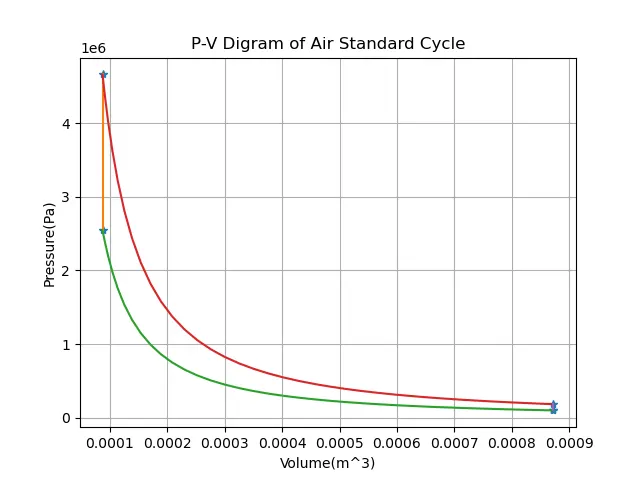
2) To plot the P-V Diagram for it.

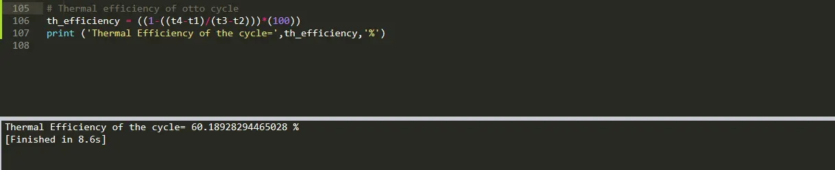
3) To find out the thermal efficiency of the cycle.

THEORY:

• OTTO CYCLE:

The Otto cycle was developed by German engineer Nikolaus Otto in 1876. This cycle is very similar to the Diesel cycle, except that the Otto cycle forms the basis of a spark-ignition (S.I.) engine, which requires a spark to begin combustion of fuel.

The Otto cycle is a description of what happens to a mass of gas as it is subjected to changes of pressure, temperature, volume, addition of heat, and removal of heat. The mass of gas that is subjected to those changes is called the system. The system, in this case, is defined to be the fluid (gas) within the cylinder. By describing the changes that take place within the system, it will also describe in inverse, the system's effect on the environment. In the case of the Otto cycle, the effect will be to produce enough net work from the system so as to propel an automobile and its occupants in the environment.

• P-V Diagram of Otto Cycle:

1) Process 0–1 a mass of air is drawn into piston/cylinder arrangement at constant pressure.

2) Process 1–2 is an adiabatic (isentropic) compression of the charge as the piston moves from bottom dead centre (BDC) to top dead centre (TDC).

3) Process 2–3 is a constant-volume heat transfer to the working gas from an external source while the piston is at top dead centre. This process is intended to represent the ignition of the fuel-air mixture and the subsequent rapid burning.

4) Process 3–4 is an adiabatic (isentropic) expansion (power stroke).

5) Process 4–1 completes the cycle by a constant-volume process in which heat is rejected from the air while the piston is at bottom dead centre.

6) Process 1–0 the mass of air is released to the atmosphere in a constant pressure process.

• ENGINE GEOMETRY:

1) Bore: The Bore is basically engine cylinder diameter in mm.

2) Stroke: The Stroke is the distance between Top Dead Centre(TDC) and Bottom Dead Centre(BDC) in mm.

3) Connecting Rod Length(Con-Rod): As the name stats it is basically the length of the connecting rod in mm.

4) Compression Ratio(Cr): The compression ratio is the ratio of the volume of the cylinder and the combustion chamber when the piston is at the bottom, and the volume of the combustion chamber when the piston is at the top.

`C_r=(V_s+V_c)/V_c`

5) Swept Volume(Vs): It is the total volume swept by the piston during its motion between TDC and BDC.

`V_s=(pi/4)*(bore)^2*stroke`

6) Clearance Volume(Vc): It is the volume obtained in the combustion chamber during the combustion stroke were the piston is very close to the TDC of the IC engine.

`V_c=V_s / (cr-1)`

7) Crank Angle(`theta`): It is the angle obtained when the crankshaft rotates during the piston motion from either TDC to BDC or BDC to TDC in degrees.

• THERMAL EFFICIENCY:

Thermal efficiency, η_th, of any heat engine is defined as the ratio of the work it does, W, to the heat input at the high temperature, Q_H.

`eta_(th)= W/Q_h`

Procedure:

• Program:

import math
import matplotlib.pyplot as plt

# Defining a Function
def engine_kinematics(bore,stroke,con_rod,cr,start_crank,end_crank):
	# Volume parameters
	V_s=math.pi*(1/4)*pow(bore,2)*stroke
	V_c=V_s/(cr-1)
	sc=math.radians(start_crank)
	ec=math.radians(end_crank)

	num_values=50

	dtheta=(ec-sc)/(num_values-1)

	V=[]

	for i in range (0,num_values):
		theta = sc + i*dtheta
		term1 = 0.5*(cr-1)
		term2 = R + 1-math.cos(theta)
		term3 = pow(R,2) - pow(math.sin(theta),2)
		term3 = pow(term3,0.5)

		V.append((1+term1*(term2-term3))*V_c)
	return V 

# Inputs
p1=101325
t1=500
gamma=1.4
t3=2300

# Geomertic parameters
bore=0.10
stroke=0.10
con_rod=0.15
cr=10
a=stroke/2
R=con_rod/a

# Volume computation
v_s = (math.pi/4)*pow(bore,2)*stroke
v_c = v_s/(cr-1)
v1 = v_c+v_s

# State point 2
v2 = v_c

# p2v2^gamma = p1v1^gamma
p2=p1*pow(v1,gamma)/pow(v2,gamma)

#p2v2/t2=p1v1/t1 | rhs = p1v1/t1 | p2v2/t2 = rhs | t2=p2v2/rhs
rhs = p1*v1/t1
t2 = p2*v2/rhs
V_compression = engine_kinematics(bore, stroke, con_rod, cr, 180, 0)

constant = p1*pow(v1,gamma)

P_compression = []

for v in V_compression:
	P_compression.append(constant/pow(v, gamma))

# State point 3
v3 = v2

#p3v3/t3 = p2v2/t2 | rhs = p2v2/t2 | p3 = rhs*t3/v3

rhs = p2*v2/t2
p3 = rhs*t3/v3
V_expansion = engine_kinematics(bore, stroke, con_rod, cr, 0, 180)

constant = p3*pow(v3,gamma)

P_expansion = []

for v in V_expansion:
	P_expansion.append(constant/pow(v, gamma))

# State point 4
v4 = v1

# p4v4^gamma = p3v3^gamma
p4 = p3*pow(v3,gamma) / pow(v4,gamma)

# p4v4/t4 = rhs
t4 = p4*v4/rhs

#Plotting 
plt.figure()
plt.plot([v1,v2,v3,v4,v1],[p1,p2,p3,p4,p1],'*')
plt.plot([v2,v3],[p2,p3])
plt.plot(V_compression,P_compression)
plt.plot(V_expansion,P_expansion)
plt.plot([v4,v1],[p4,p1])
plt.xlabel('Volume(m^3)')
plt.ylabel('Pressure(Pa)')
plt.title('P-V Digram of Air Standard Cycle')
plt.grid('on')
plt.savefig('P-V Diagram')
plt.show()


# Thermal efficiency of otto cycle
th_efficiency = ((1-((t4-t1)/(t3-t2)))*(100))
print ('Thermal Efficiency of the cycle=',th_efficiency,'%')

• Stepwise Explanation:

1) We first import the math library and plot library for performing mathematical operations and plotting the graphs.

2) We define a function that contains parameters used in the engine kinematics. Here, we have calculated the swept volume and clearance volume . Then using the for loop we have tried to spilt the equation in three terms i.e., term1 , term2 , term3 .

3) We then inputs the values of bore, stroke, connecting rod length, crank pin radius, Gamma and Compression ratio.

4) We also inputs the values of Pressure (p1) and Temperature (t1) at state point 1 and Temperature (t3) is also inputed since the temperature during expansion is high.

5) We calculate the Pressure (p), Volume(v) and Temperature(t) at all the state points using the ideal gas equation.

6) We use For loop to get set of during Compression and Expansion process.

7) We then plot the graph for the air standard cycle using the plot command. We also save the plot in the image format using the Savefig command.

8) We then calculate the Thermal Efficiency of the Air Standard Cycle using the following formula.

Thermal Effieciency (ηth">ηthηth) = 1-(t4-t1t3-t2)">1−((t4−t1)/(t3−t2))*100

9) We finally use the print command to show the Thermal Efficiency as output.

Results and Discussion:

1) We run the program using the Ctrl+B and we find that there are no errors in the program and the program has ran succesfully.

2) We get the thermal efficiency of the otto cycle = 60.189 % as shown in the image given below.

3) We also get the plot of the air standard cycle or ottto cycle as shown in the image given below.