Week 4.1 - Genetic Algorithm
AIM
- To write a code in MATLAB to optimise the stalagmite function and find the global maxima of the function
- To understand the concept of genetic algorithm
THEORY
Genetic Algorithm (GA) is a search-based optimization technique based on the principles of Genetics and Natural Selection. This algorithm reflects the process of natural selection where the fittest individuals are selected for reproduction in order to produce offspring of the next generation. It is frequently used to find optimal or near-optimal solutions to difficult problems which otherwise would take a lifetime to solve. Genetic algorithms are commonly used to generate high-quality solutions to optimization and search problems by relying on biologically inspired operators such as mutation, crossover and selection.
The main characteristics of a genetic algorithm are as follows:
- The genetic algorithm works with a coding of the parameter set, not the parameters themselves.
- The genetic algorithm initiates its search from a population of points, not a single point.
- The genetic algorithm uses payoff information, not derivatives.
- The genetic algorithm uses probabilistic transition rules, not deterministic ones.
Advantages
- The concept is easy to understand.
- GA search from a population of points, not a single point.
- GA use payoff (objective function) information, not derivatives.
- GA supports multi-objective optimization.
- GA use probabilistic transition rules, not deterministic rules.
Disadvantages
- GA is computationally expensive
- Time consuming
- GA implementation is still an art
- In GA designing an objective function mand getting the operators right can be difficult
Applications of GA
- To solve optimization problems
- Image processing
- Code breaking
- learning robot beahviour
- Vehicle routing problems
- DNA analysis
- Multimodal optimization
- Plant floor layout etc
Syntax of GA
x = ga(fun,nvars,A,b,Aeq,Beq,lb,ub,nonlcon,IntCon,options)
where
fun = objective function
nvars = no. of variables used
A = used if inequality exist in the function
b = used if inequality exist in the function
Aeq = used if inequality exist in the function
Beq = used if inequality exist in the function
lb = lower limit
ub = upper limit
nonlcon = accepts x and returns vectors C and Ceq, representing the nonlinear inequalities and equalities respectively
IntCon = take integer values
Options = allows to add extra parameters
Function code
function [F]= stalagmite_fun(input_vector)
x=input_vector(1);
y=input_vector(2);
f1=(sin((5.1*pi*x+0.5)))^6;
f2=((sin(5.1*pi*y+0.5)))^6;
f3= exp((-4*log(2)*((x-0.0667)^2)/0.64));
f4=exp((-4*log(2)*((y-0.0667)^2)/0.64));
F=(f1*f2*f3*f4*-1);
end
Genetic algorithm always finds the minima of the given function, so negative sign is used so that the plot is reversed to obtain the maxima.
Main code
clear all
close all
clc

%defining search space
x = linspace(0,0.6,150);
y = linspace(0,0.6,150);

%creating a 2Dimensional mesh
[xx,yy] = meshgrid(x,y);

num_cases = 50;

%evaluating the stalagmite function
for i = 1:length(xx)
    for j = 1:length(yy)
        input_vector(1) = xx(i,j);
        input_vector(2) = yy(i,j);
        f(i,j) = stalagmite(input_vector);
    end
end


tic %study time counting starts
%unbounded statistical behaviour
for i =1:num_cases
    [inputs1,fopt1(i)] = ga(@stalagmite,2); %GA function is used to run stalagmite data
    xopt(i) = inputs1(1);
    yopt(i) = inputs1(2);
end

study1_time = toc %study time counting ends

figure(1)
subplot(2,1,1)
hold on
surfc(xx,yy,f) %generates stalagmite function
xlabel(x)
ylabel(y)
shading interp %to create smooth curve surface
plot3(xopt,yopt,fopt1,'marker','o','markersize',5,'markerfacecolor','r')
title('unbounded inputs')
subplot(2,1,2)
plot(fopt1)
xlabel('iterations')
ylabel('function maxima')

%bounded statistical behaviour
tic;
for i =1:num_cases
    [inputs2,fopt2(i)] = ga(@stalagmite,2,[],[],[],[],[0;0],[0.6;0.6]);
    xopt(i) = inputs2(1);
    yopt(i) = inputs2(2);
end

study2_time = toc

figure(2)
subplot(2,1,1)
hold on
surfc(xx,yy,f)
shading interp
plot3(xopt,yopt,fopt2,'marker','o','markersize',5,'markerfacecolor','r')
title('bounded inputs')
subplot(2,1,2)
plot(fopt2)
xlabel('iterations')
ylabel('function maxima')

%study 3 increasing ga iterations
options = optimoptions('ga');
options = optimoptions(options,'populationSize',200);  %population size is increased to converge to the global maxima

tic;
for i =1:num_cases
    [inputs3,fopt3(i)] = ga(@stalagmite,2,[],[],[],[],[0;0],[0.6;0.6],[],[],options);
    xopt(i) = inputs3(1);
    yopt(i) = inputs3(2);
end

study3_time = toc

figure(3)
subplot(2,1,1)
hold on
surfc(xx,yy,f)
shading interp
plot3(xopt,yopt,fopt3,'marker','o','markersize',5,'markerfacecolor','r')
title('bounded inputs with increased population size')
subplot(2,1,2)
plot(fopt3)
xlabel('iterations')
ylabel('function maxima')
The x and y inputs is defined using the linspace command. Then mesh is created from the two vectors using the meshgrid command.
The number of cases is mentioned which is used for the iteration process. The stalagmite function which is defined separately is called into the main program.
GA calculates the values of the fitness function at each point in the mesh.
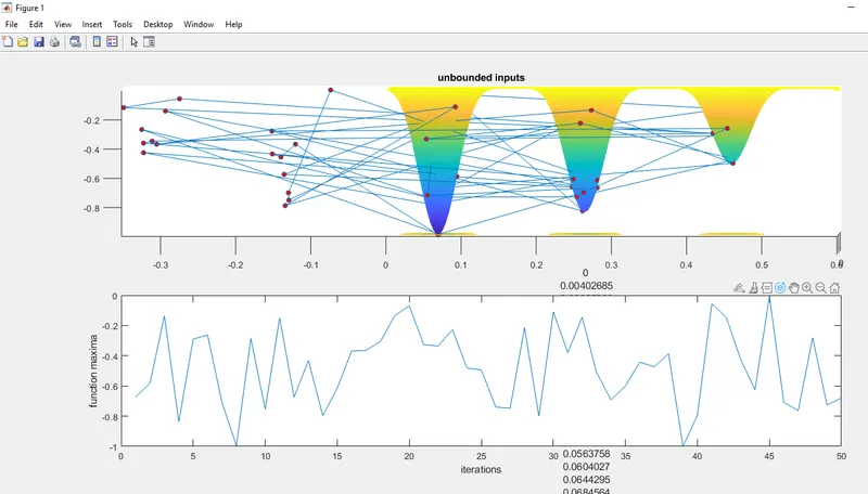
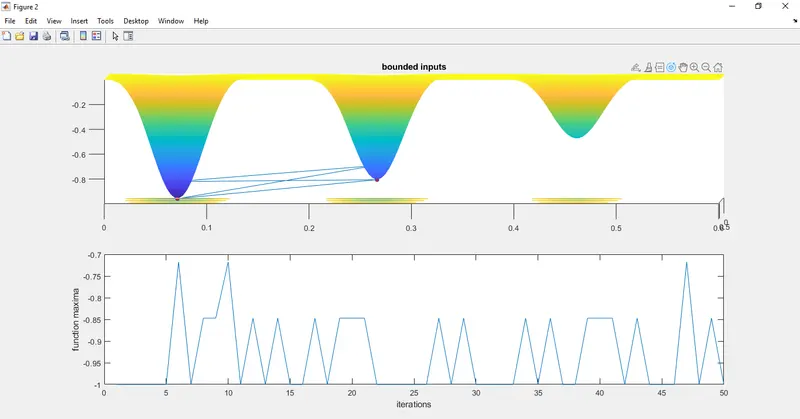
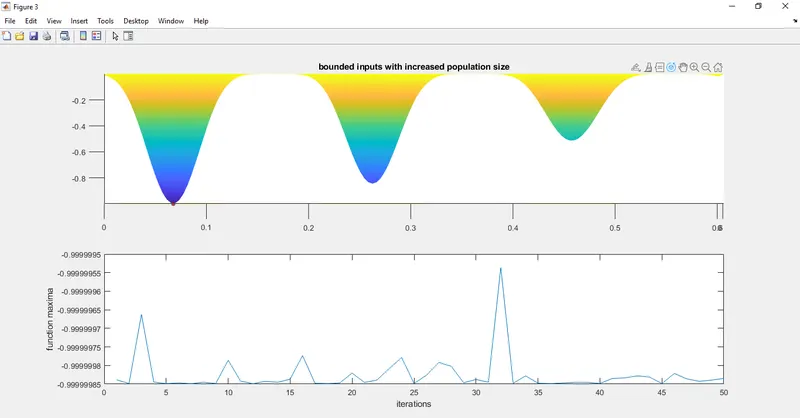
Then coding for 3 studies are done. The first one with unbounded inputs, the second study with bounded inputs and the third study with increased population size.
Graphs for all three studies are plotted. The results are plotted using surfc and plot commands.
RESULTS
Study 1- with unbounded inputs:
study1_time =3.0779s
Study 2 - with bounded inputs
By dedfining the boundaries, the search space is reduced. So the algorithm has to find the maxima only within the limits.
study2_time = 3.5816s
study 3 - Bounded inputs with increased population size
In this case the population size in increased, to converge to the global maxima.
study3_time = 9.9174s
REFERENCES
https://in.mathworks.com/discovery/genetic-algorithm.html
https://en.wikipedia.org/wiki/Genetic_algorithm
https://www.sciencedirect.com/topics/engineering/genetic-algorithm