Week 1: Channel flow simulation using CONVERGE CFD
AIM
To simulate the channel flow using Converge
OBJECTIVES
1. For this challenge, we will be setting up a channel flow tutorial.
2. Set up the case in CONVERGE
3. Make sure the inlet pressure and initial pressure are the same.
4. Once the base setup is ready, run the case for three different base mesh sizes
i.e Run 3 simulations and compare the results between all the 3 simulations.
3 different base mesh sizes are,
- dx = 2e-4m, dy = 2e-4m, dz = 2e-4m
- dx = 1.5e-4m, dy = 1.5e-4m, dz = 1.5e-4m
- dx = 1.0e-4m, dy = 1.0e-4m, dz = 1.0e-4m (If this is too much for your PC, use 1.2e-4m)
THEORY
Channel flow
Channel flow is an internal flow in which the confining walls change the hydrodynamic structure of the flow from an arbitrary state at the channel inlet to a certain state at the outlet. The flow through a rectangular channel is characterised by zero velocity at the wall due to no slip condition.
Flow simulation is a form of computational fluid dynamics which digitally replicates flows in surface water or collection systems. Performing flow simulation allows for the prediction and analysis of how a flow might be impacted by complex geometry in an operational environment.
SIMULATION PROCEDURE
- Setting up the case in converge
- Running the simulation in cygwin
- Post convert using cygwin/converge
- Post processing in paraview
The first step is case setup in converge. Open converge and then create the geometry.
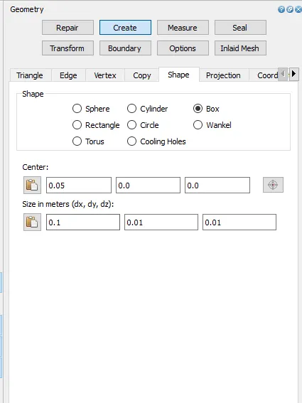
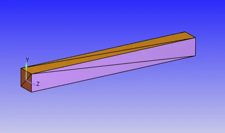
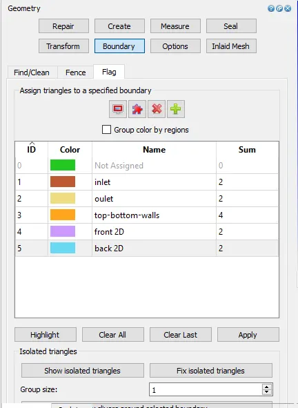
Create the boundaries and name them
The orientation of normals should be checked such that it should be pointing inwards.
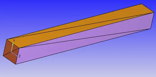
After creating the geometry the next step is to setup the case
Inorder to run a steady state simulation firstly under application type in the setup tree, a time based simulation must be selected.
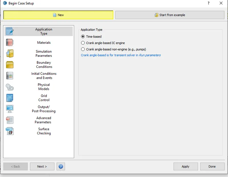
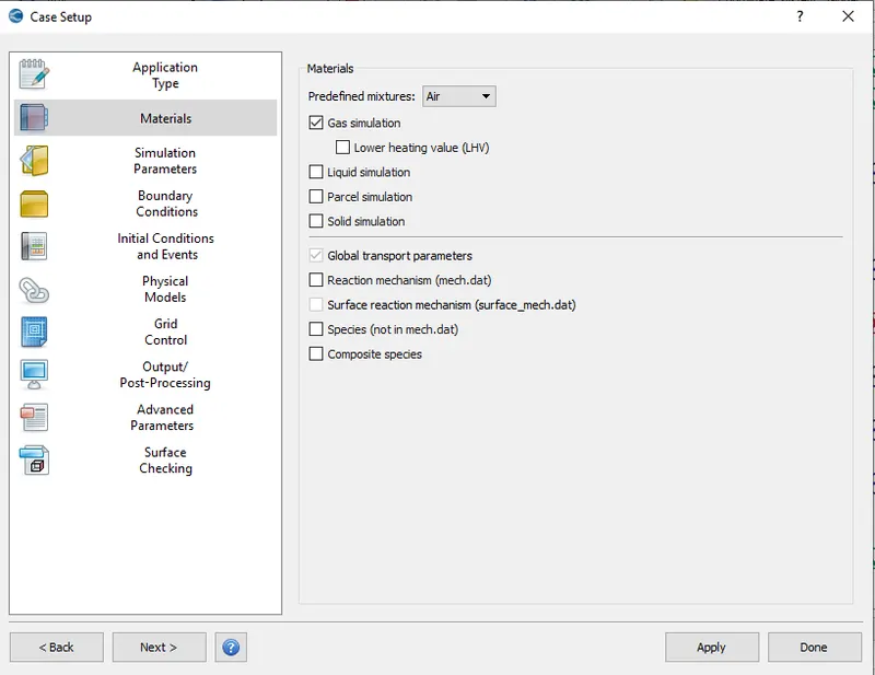
Next in materials, uncheck the reaction mechanism since we are not dealing with any reactions in the channel flow. In predefined mixtures select air and choose gas simulation.
Choose the default properties in the gas simulation.
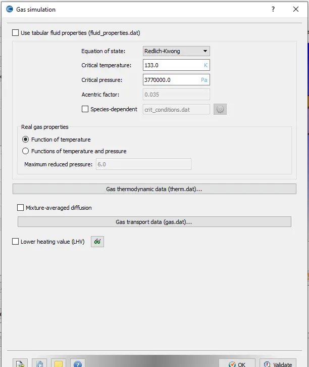
Default properties retained
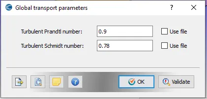
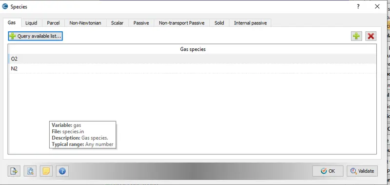
In species select O2 and N2, since air is composed of nitrogen and oxygen.
The next one in the case setup tree is the simulation parameters.
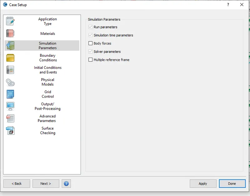
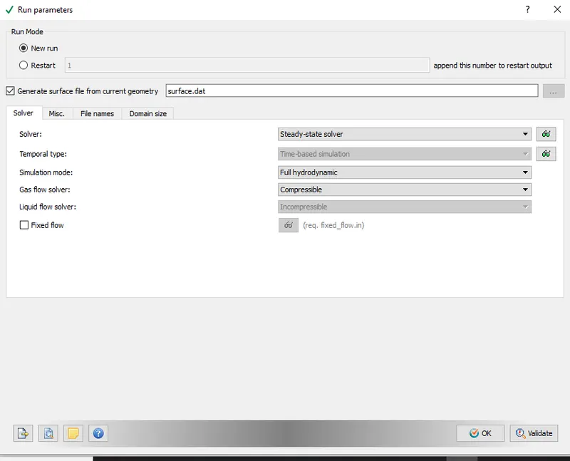
Next in the run parameters tab, select steady state solver.
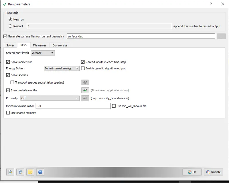
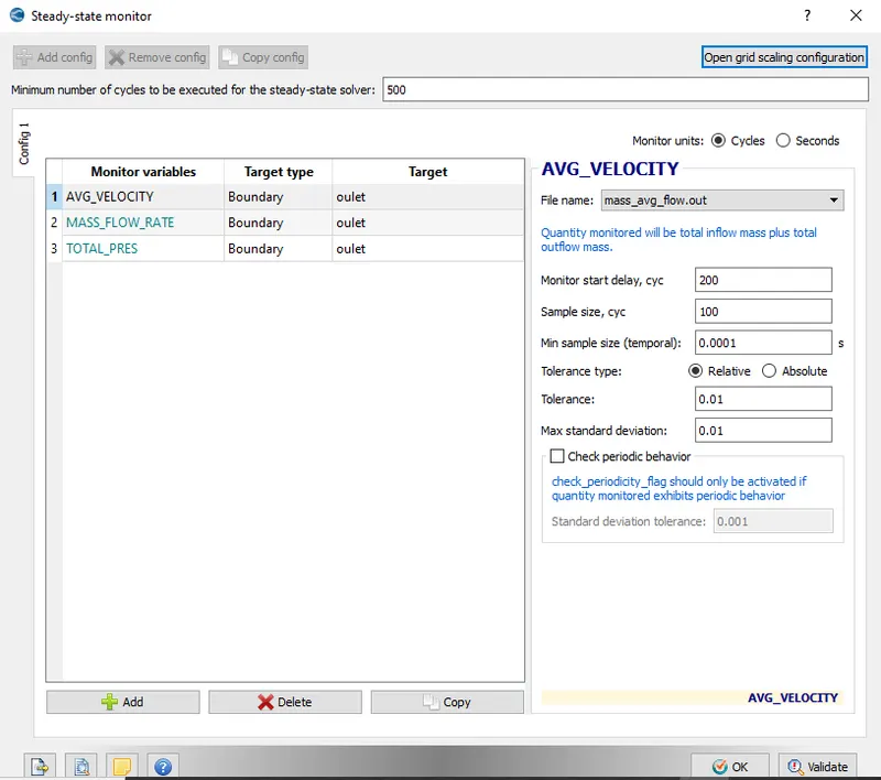
The steady state monitor is a mandatory option for steady state simulations in order to assess convergence of the solution. Turn on steady state monitor.
Select the variable to be monitored in the steady state monitor tab. Then select the boundary at which the variable needs to be monitored. Choose oulet because an inlet boundary condition was given.
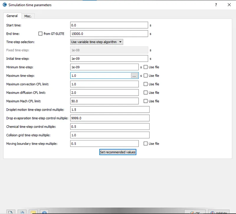
Give the simulation time parameters
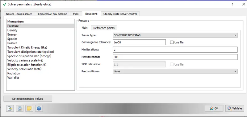
Solver parameters:
Solver scheme - PISO
Solver type - density based
Pressure preconditioner - none
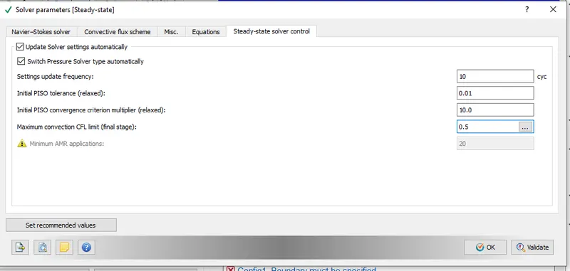
In solver parameters the maximum convection CFL limit should be less than one.
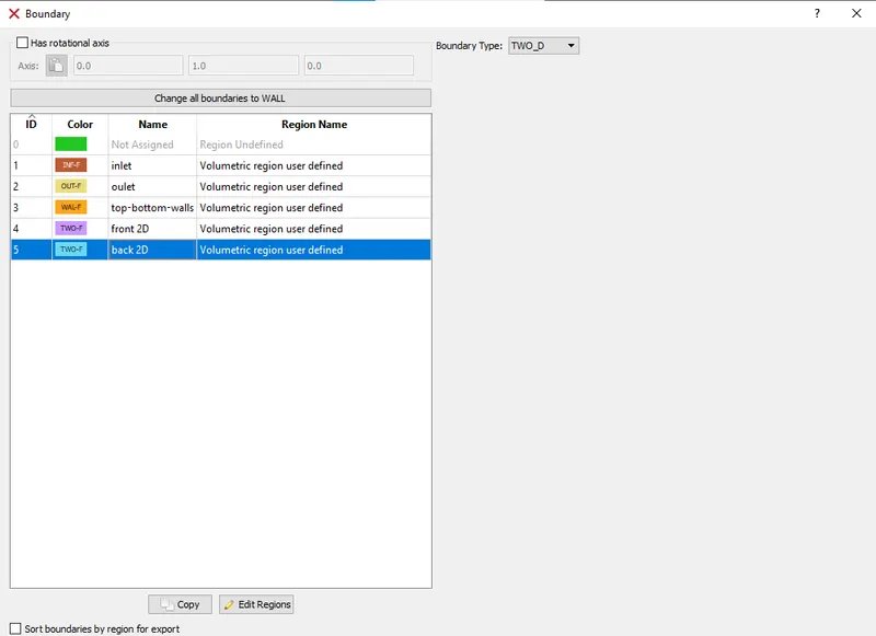
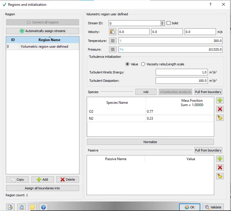
Give the boundary conditions for each boundary as shown below
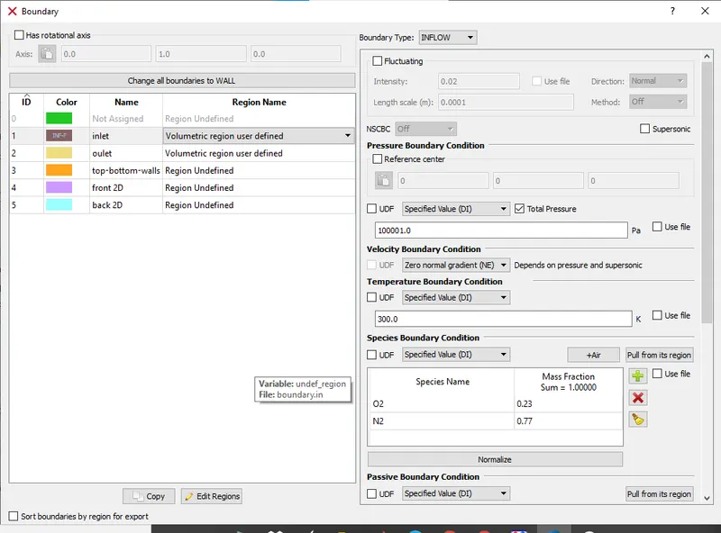
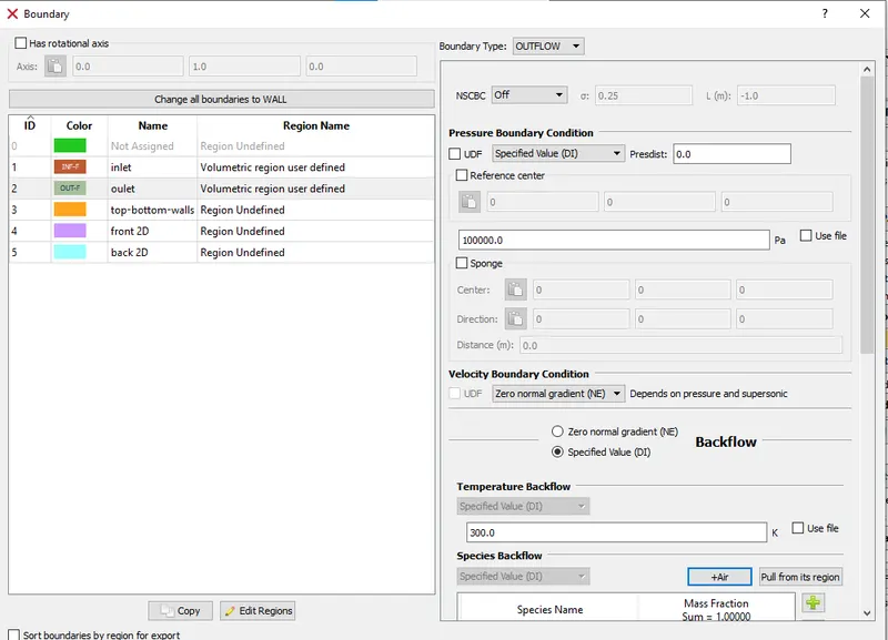
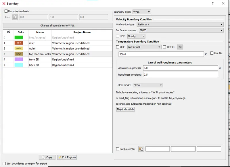
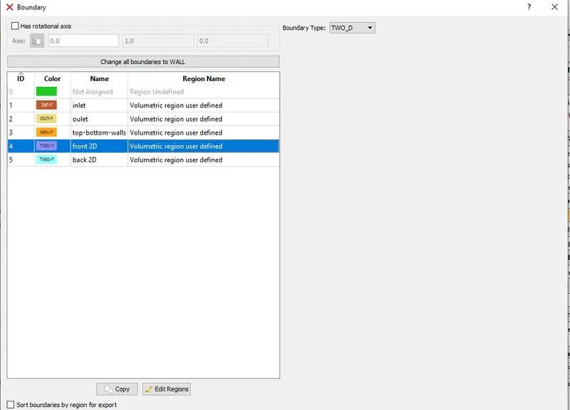
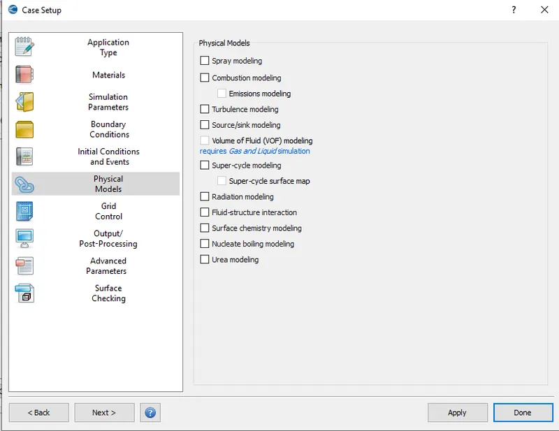
In physical models turn off turbulence modeling.
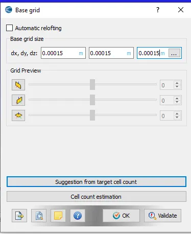
In base grid tab, the mesh sizes is to be entered.
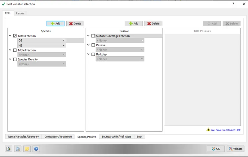
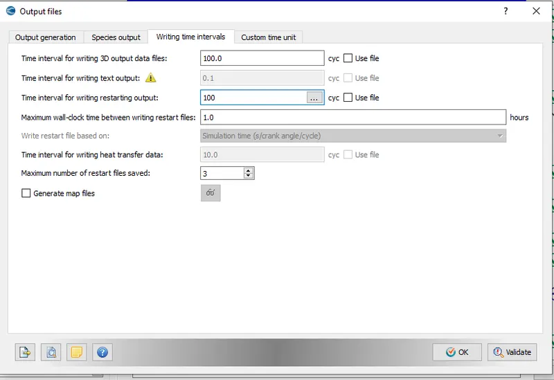
Set the frequency of generation of output files
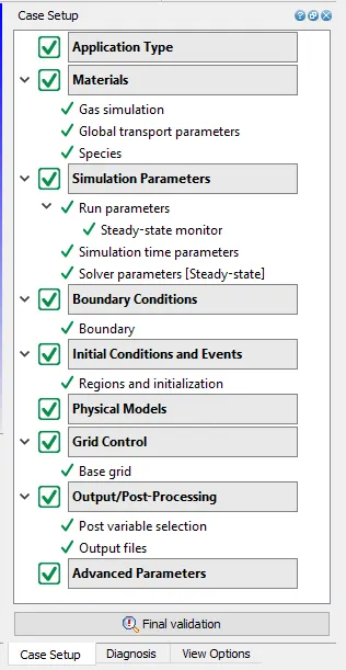
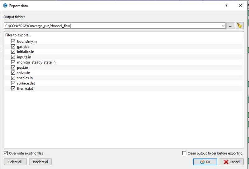
Once the case setup is completed, export the input files into a required directory.
 Then launch cygwin and navigate to the directory through CYGWIN in which all input files has been exported and then enter the command to run the simulation. After that post convert using converge and post process the results in paraview.
RESULTS
Case 1
Mesh size, dx = 2e-4m, dy = 2e-4m, dz = 2e-4m
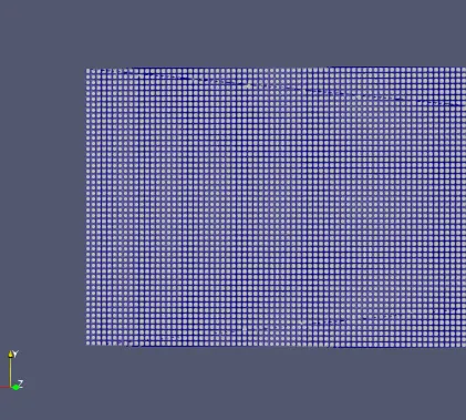
Mesh
Velocity contour
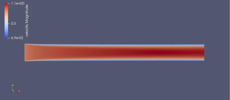
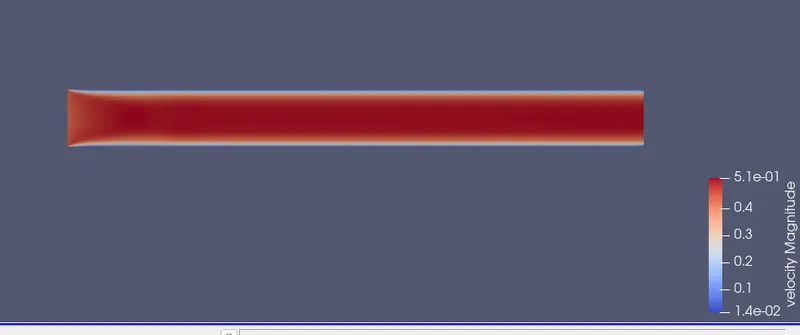
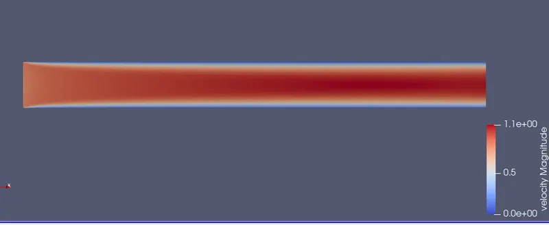
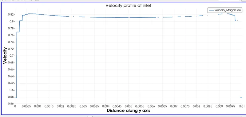
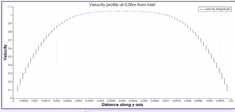
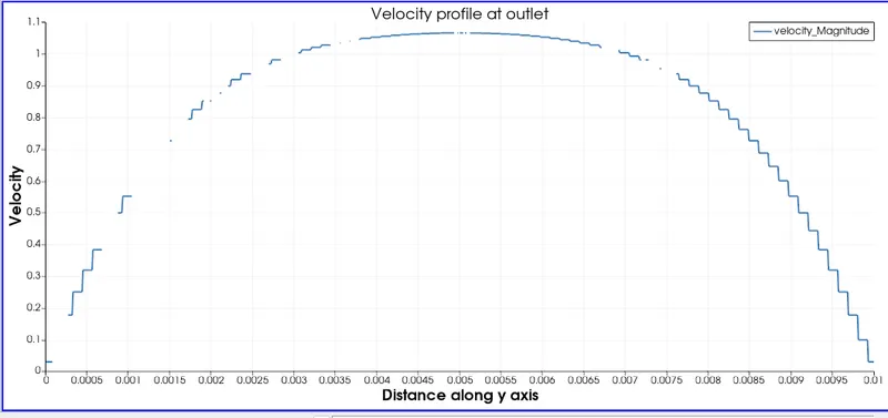
At the inlet the velocity is uniform along the y axis. As the flow proceeds through the channel the velocity of the fluid is minimum along the wall, this is due to the no slip boundary condition. In fluid dynamics, the no-slip condition for viscous fluids assumes that at a solid boundary, the fluid will have zero velocity relative to the boundary. The fluid velocity at all fluid–solid boundaries is equal to that of the solid boundary. In the boundary layer the effect of viscosity is dominant. For the flow away from the wall the effect of inertia is dominant. From the plot we can see that the velocity is maximum along the centre of the channel. This can be understood from the velocity profile given below.
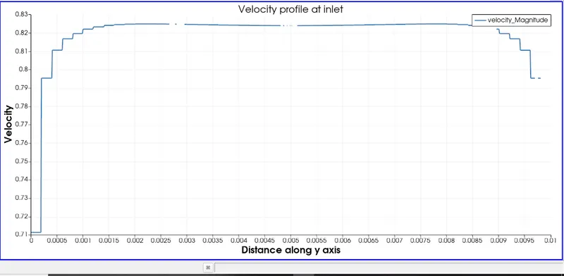
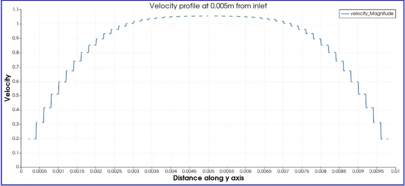
Velocity profile along the length of the channel
At inlet:
At 0.05m from inlet:
At outlet:
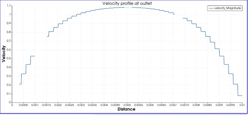
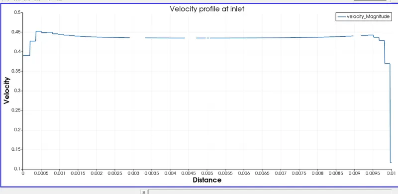
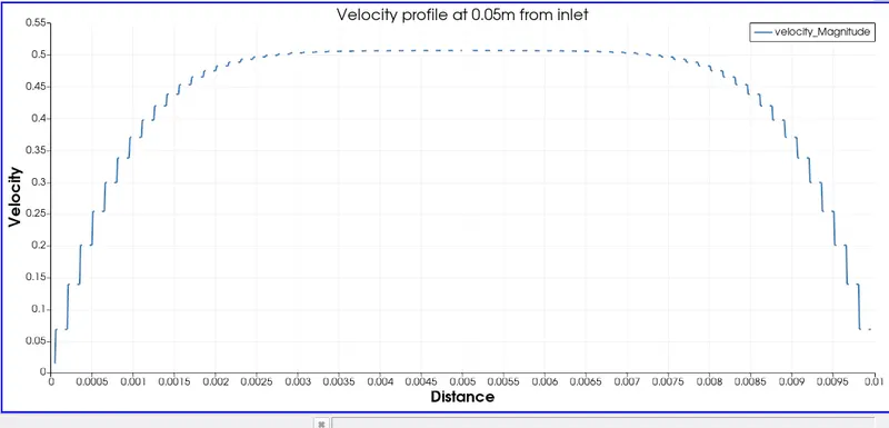
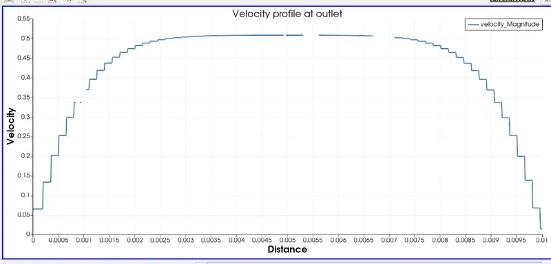
At the entrance of the pipe the velocity profile is flat. As the flow move across the channel the velocity profile develops a parabolic shape.
Mass flow rate
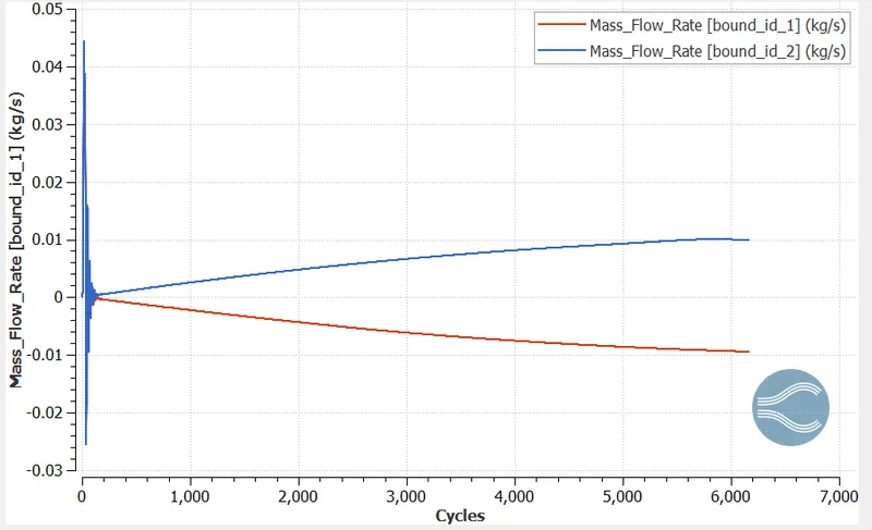
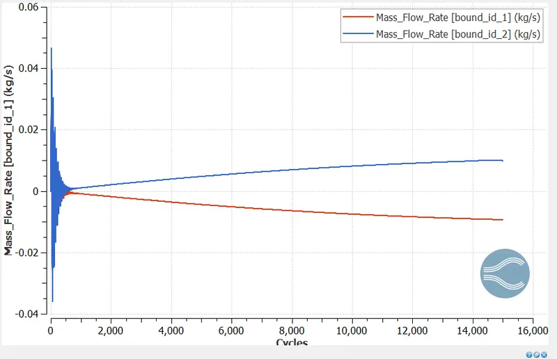
From the graph it is clear that mass is conserved. That is mass flowing into the channel is coming out of it.
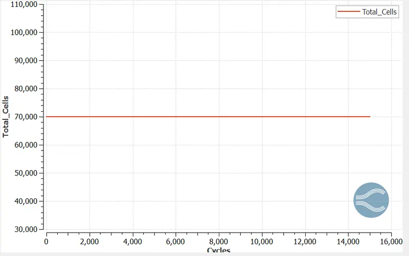
Total cell count
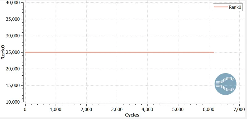
Total cell count = 25000
Total pressure
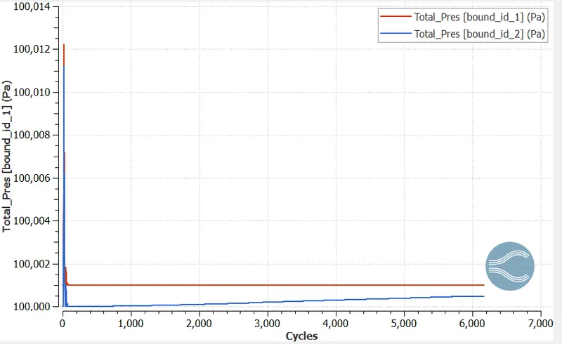
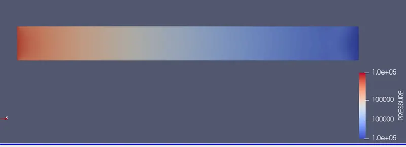
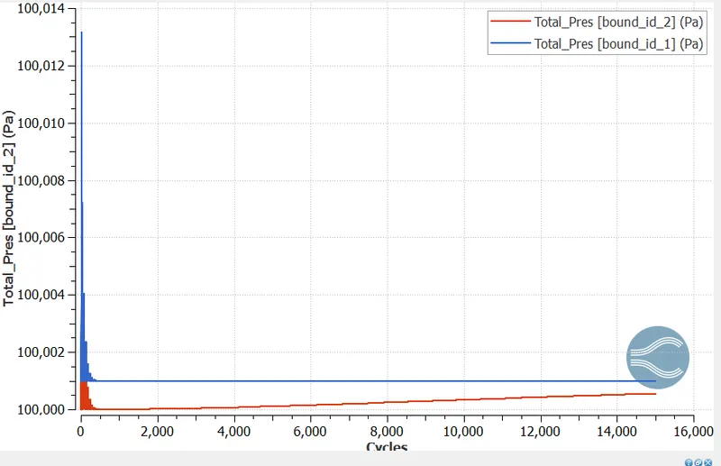
From the plot we can see that the inlet pressure remains constant, but the outlet pressure slightly increases.
Pressure contour
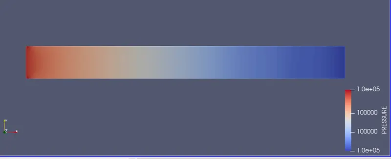
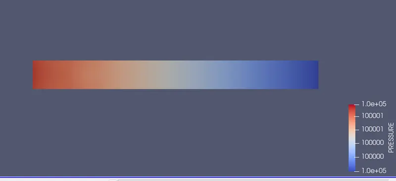
Pressure difference is the driving potential of the flow. The inlet pressure was given as 100001Pa and outlet pressure as 100000Pa. Fluid flow requires a pressure gradient between two points such that flow is directly proportional to the pressure differential. Higher pressure differences will drive greater flow rates. The pressure gradient establishes the direction of flow.
Velocity animation
https://drive.google.com/file/d/1vxkRJyDWfNOyGMT5wMhoFD08HawBoliT/view?usp=sharing
Case 2
Mesh size, dx = 1.5e-4m, dy = 1.5e-4m, dz = 1.5e-4m
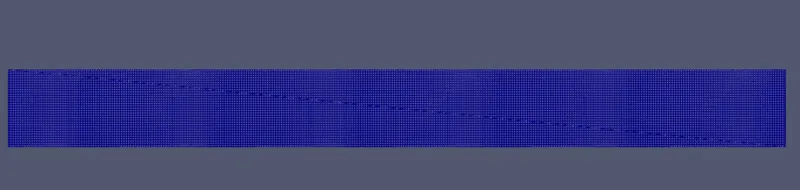
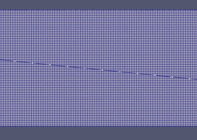
Mesh
Velocity contour
Pressure contour
Mass flow rate
Velocity profiles along the length of the channel
At inlet
At 0.05m from inlet
At outlet
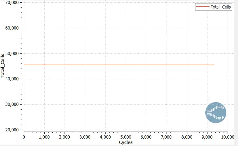
Total cell count
Velocity animation
https://drive.google.com/file/d/1uN8bes-Bi74IMWBn-X5LP_f_nyTlGN82/view?usp=sharing
Case 3
Mesh size, dx = 1.2e-4m, dy = 1.2e-4m, dz = 1.2e-4m
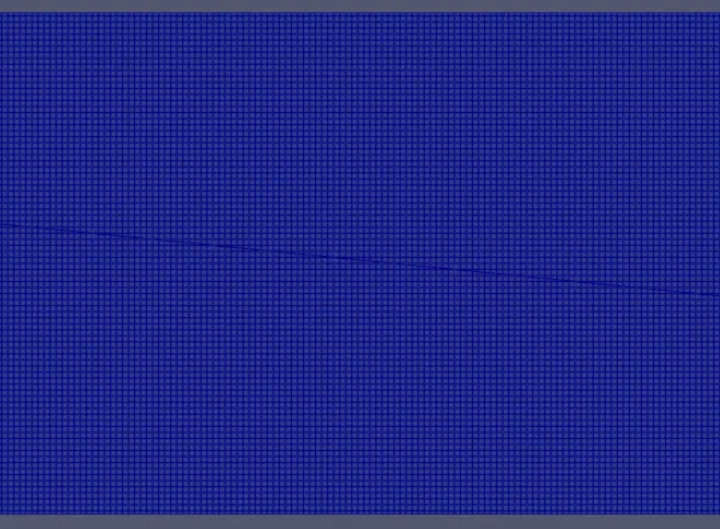
Mesh

Velocity contour
Pressure contour
Mass flow rate
Velocity profiles along the length of the channel
At inlet
At 0.05m from inlet
At outlet
Total pressure
Total cell count
Velocity animation
https://drive.google.com/file/d/1Q70hwKA272lUgKgqziwCE0S5p-fy_0tT/view?usp=sharing
CONCLUSION
- Pressure is the driving force of the flow through the channel.
- Velocity contours depicts the formation of noslip condition at the wall.
- Mass flow rate graphs confirm the conservation of mass (The plots are inverse of each other).
- With mesh refinement the computational time increases and produces better results.