Week 5: Prandtl Meyer Shock problem
AIM
To simulate prandtl meyer shock using converge
OBJECTIVES
- To study the prandtl meyer shock wave
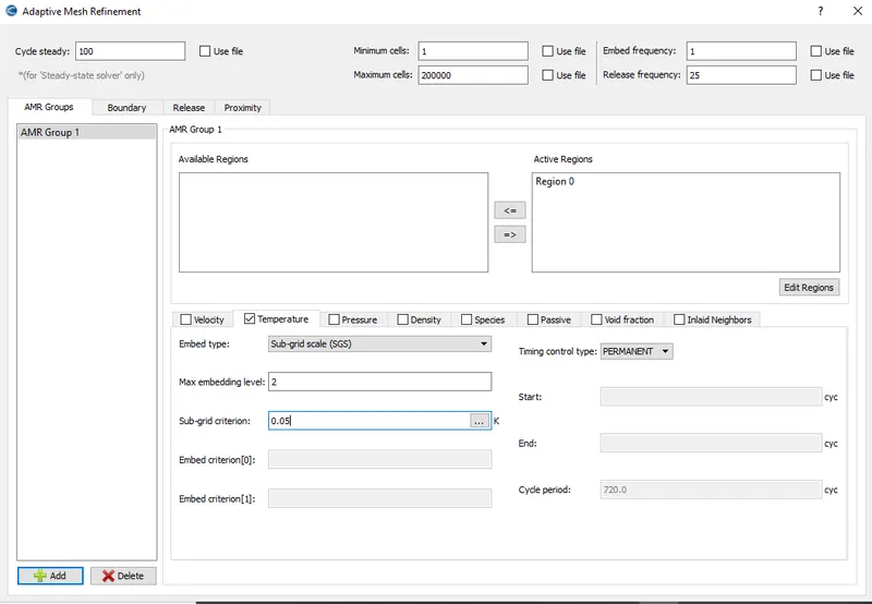
- Study the effect of SGS parameter on shock location
THEORY
Shock wave
In physics, a shock wave, or shock, is a type of propagating disturbance that moves faster than the local speed of sound in the medium. Like an ordinary wave, a shock wave carries energy and can propagate through a medium but is characterized by an abrupt, nearly discontinuous, change in pressure, temperature, and density of the medium. For the purpose of comparison, in supersonic flows, additional increased expansion may be achieved through an expansion fan, also known as a Prandtl–Meyer expansion fan. The accompanying expansion wave may approach and eventually collide and recombine with the shock wave, creating a process of destructive interference. The sonic boom associated with the passage of a supersonic aircraft is a type of sound wave produced by constructive interference.
Unlike solitons (another kind of nonlinear wave), the energy and speed of a shock wave alone dissipates relatively quickly with distance. When a shock wave passes through matter, energy is preserved but entropy increases. This change in the matter's properties manifests itself as a decrease in the energy which can be extracted as work, and as a drag force on supersonic objects; shock waves are strongly irreversible processes.
Prandtl–Meyer expansion fan
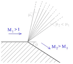
A supersonic expansion fan, technically known as Prandtl–Meyer expansion fan, a two-dimensional simple wave, is a centered expansion process that occurs when a supersonic flow turns around a convex corner. The fan consists of an infinite number of Mach waves, diverging from a sharp corner. When a flow turns around a smooth and circular corner, these waves can be extended backwards to meet at a point.
Each wave in the expansion fan turns the flow gradually (in small steps). It is physically impossible for the flow to turn through a single "shock" wave because this would violate the second law of thermodynamics. Across the expansion fan, the flow accelerates (velocity increases) and the Mach number increases, while the static pressure, temperature and density decrease. Since the process is isentropic, the stagnation properties (e.g. the total pressure and total temperature) remain constant across the fan.
Shock flow boundary conditions
Boundary conditions define the inputs of the simulation model. Some conditions, like velocity and volumetric flow rate, define how a fluid enters or leaves the model. Other conditions, like film coefficient and heat flux, define the interchange of energy between the model and its surroundings. Boundary conditions connect the simulation model with its surroundings. Without them, the simulation is not defined, and in most cases cannot proceed. Most boundary conditions can be defined as either steady-state or transient. Steady-state boundary conditions persist throughout the simulation. Transient boundary conditions vary with time, and are often used to simulate an event or a cyclical phenomena.
There are five types of boundary conditions: Dirichlet, Neumann, Robin, Mixed, and Cauchy, within which Dirichlet and Neumann are predominant.
The Dirichlet boundary condition is a type of boundary condition, when imposed on an ordinary or a partial differential equation, it specifies the values that a solution needs to take along the boundary of the domain.
The Neumann boundary condition is a type of boundary condition, when imposed on an ordinary or a partial differential equation, the condition specifies the values of the derivative applied at the boundary of the domain.
The Robin boundary condition is a type of boundary condition, when imposed on an ordinary or a partial differential equation, it is a specification of a linear combination of the values of a function and the values of its derivative on the boundary of the domain.
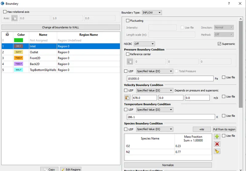
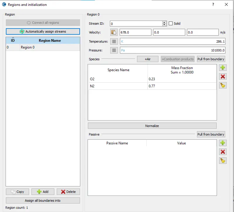
For shock flow (supersonic flow) the properties at the inlet are known, so their values has to be specified. At the outlet all the values are extrapolated from the interior. Therefore at the inlet dirichlet boundary condition and at the outlet neumann boundary condition is provided.
SIMULATION PROCEDURE
- Setting up the case in converge
- Running the simulation in cygwin
- Post convert using cygwin/converge
- Post processing in paraview
The first step is case setup in converge. Open converge and then import the geometry.
Name the boundaries
The orientation of normals should be checked such that it should be pointing inwards.
Then run a diagnosis check to find if there are any errors.
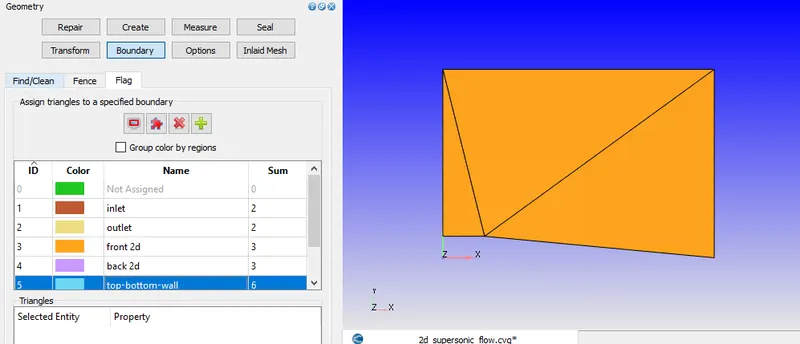
Geometry preparation is completed. The next step is case setup.
Inorder to run a steady state simulation firstly under application type in the setup tree, a time based simulation must be selected.
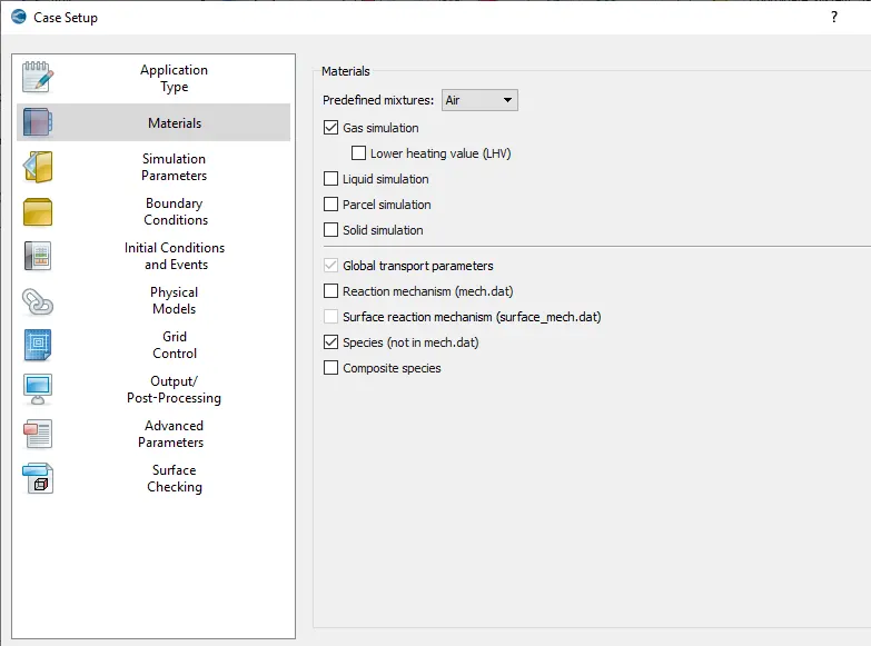
In materials turn on species and in predefined mixtures select air.
In gas simulation and global transport properties, default properties are maintained.
In species tab, add O2 and N2.
The next one in the case setup tree is the simulation parameters. In the run parameters tab, select steady state solver.
The steady state monitor is a mandatory option for steady state simulations in order to assess convergence of the solution. Turn on steady state monitor.
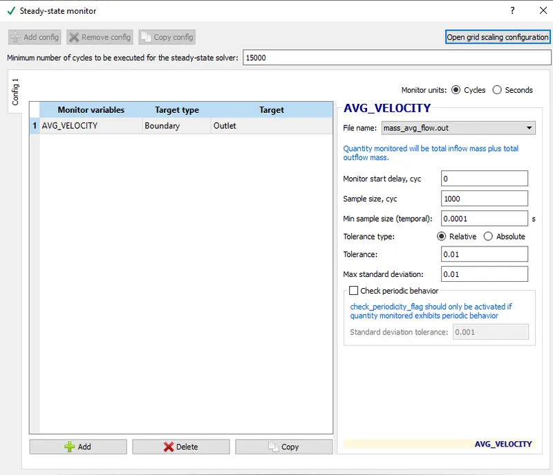
Set the simulation time parameters
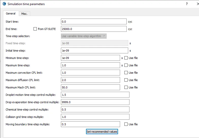
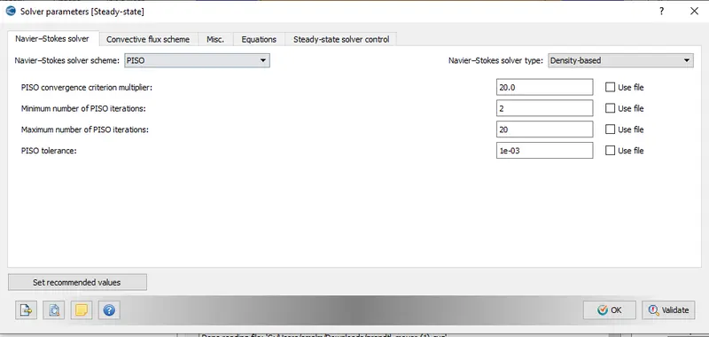
Solver parameters:
Solver scheme - PISO
Solver type - density based
Pressure preconditioner - none
The maximum convection CFL limit should be less than one.
Give the boundary conditions as given below.
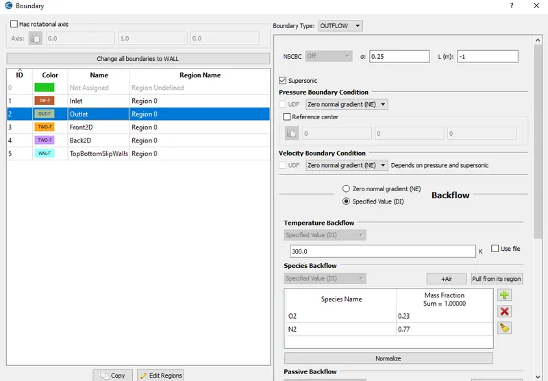
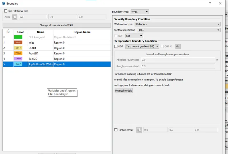
Front and back walls is set to 'TWO_D'.
In grid control turn on Adaptive mesh refinement
The base grid size is set to 0.8m
Set the frequency of generation of output files.
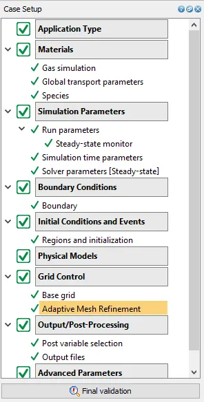
Once the case setup is completed, export the input files into a required directory. Then launch cygwin and navigate to the directory through CYGWIN in which all input files has been exported and then enter the command to run the simulation ' mpiexec.exe -n 1 converge.exe restricted'. After that post convert using converge and post process the results in paraview.
RESULTS
Study of effect of SGS parameter on shock location
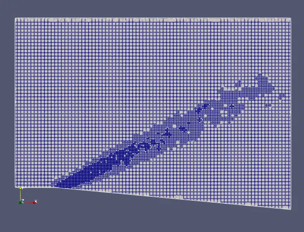
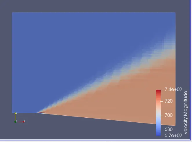
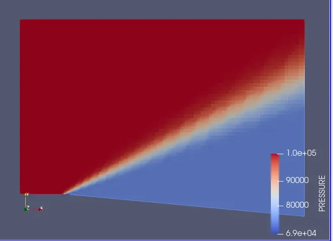
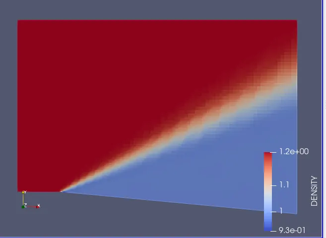
Case 1
Sub grid-criterion = 0.05
Mesh
Velocity contour
Pressure contour
Density contour
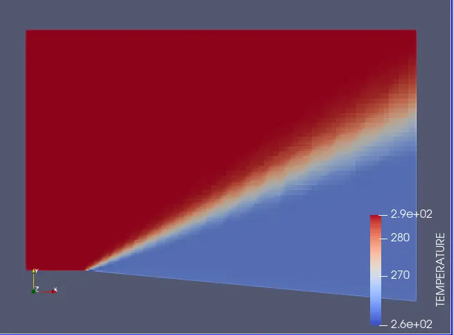
Temperature contour
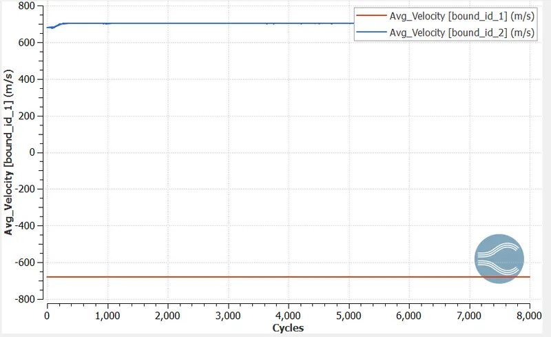
Average velocity plot
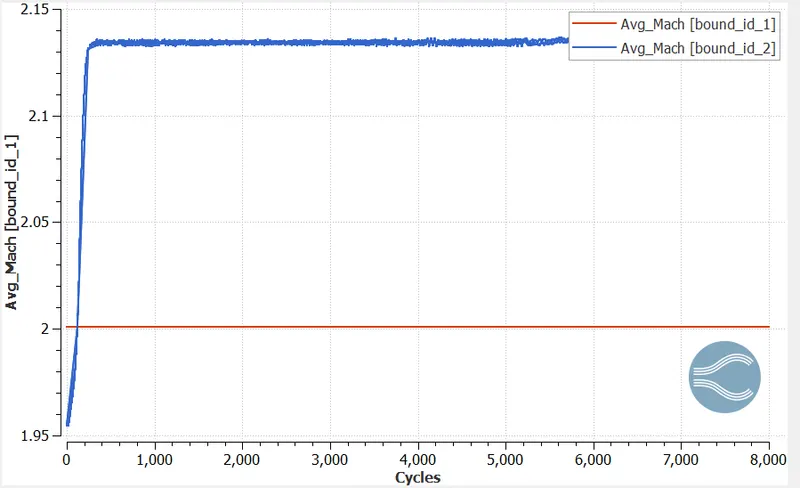
Mach number plot
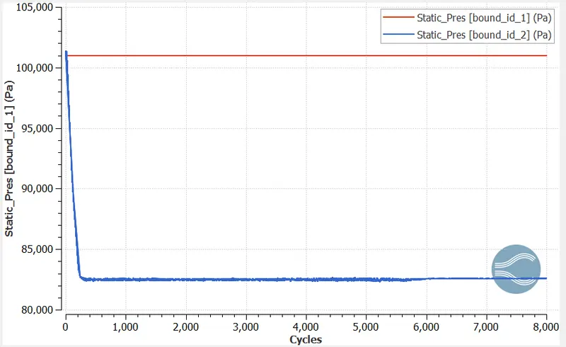
Static pressure plot
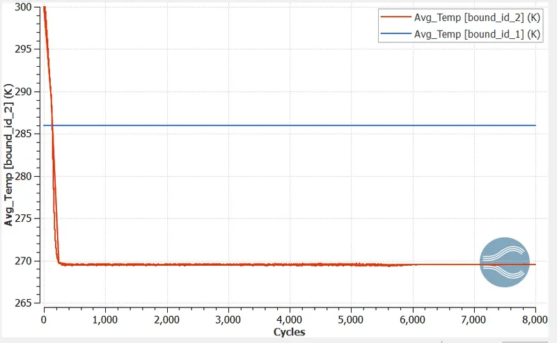
Average temperature plot
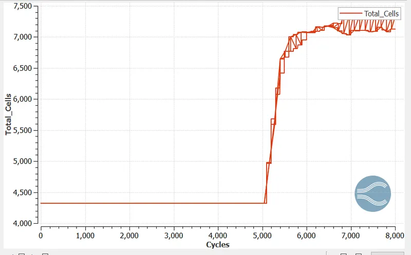
Total cell count plot
The animation video link is provided below:
https://drive.google.com/file/d/1oX2_ClzVXiyG8PWJl8zv2jxzy1R-WxId/view?usp=sharing
Case 2
Sub grid-criterion = 0.0025
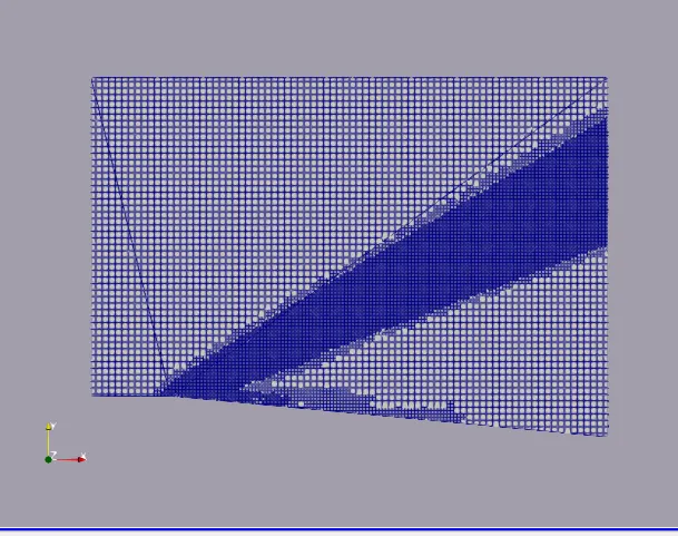
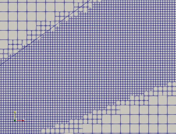
Mesh
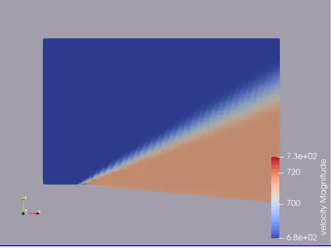
Velocity contour
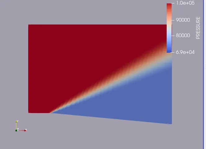
Pressure contour
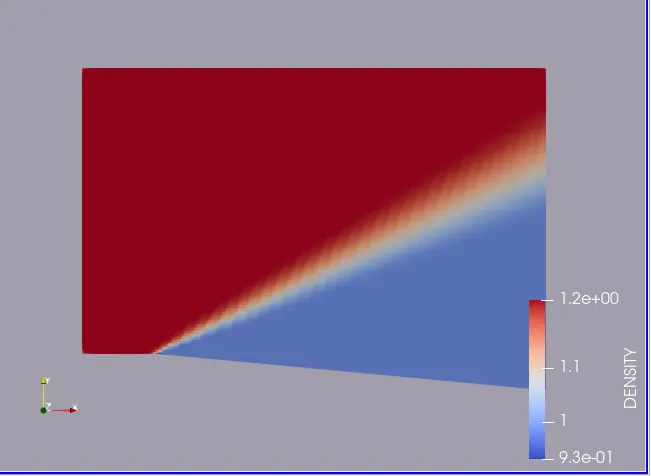
Density contour
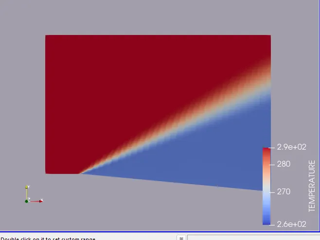
Temperature contour
Static pressure plot
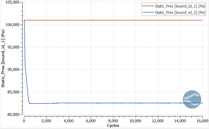
Temperature plot
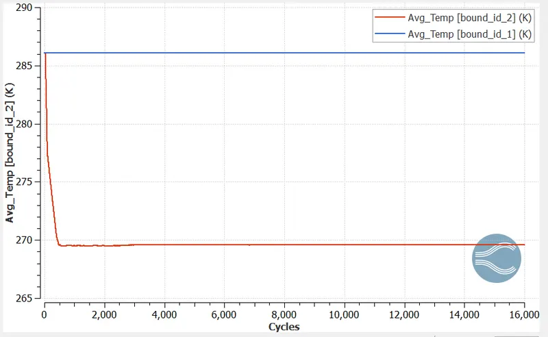
Mach number plot
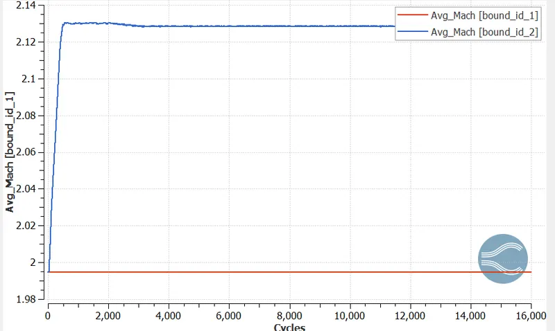
Total cell count plot
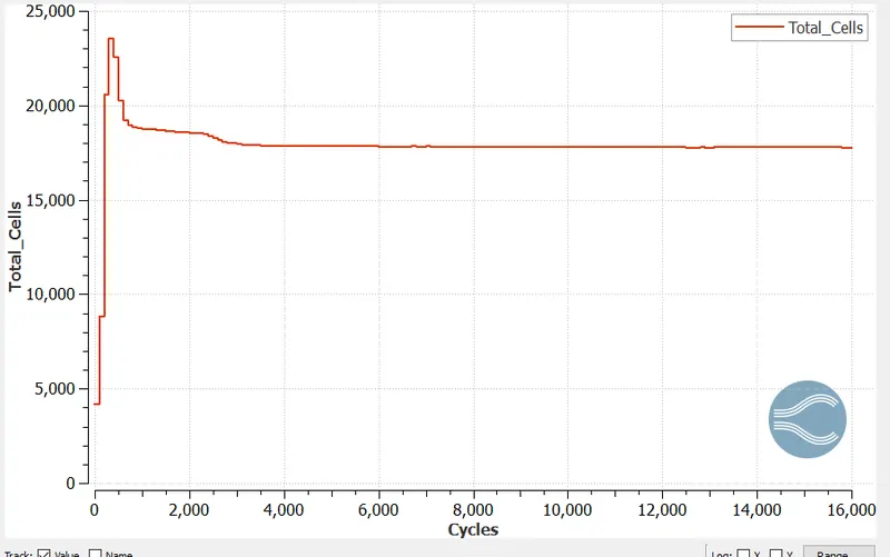
The animation video link is provided below:
https://drive.google.com/file/d/1b8WYRlr-hwFBQSiKEPmDfiyAe2_nDk5C/view?usp=sharing
Effect of SGS parameter on shock location
- From the results, it is clear that as the SGS value decreases the mesh refinement increases.
- In the second case where the SGS value is very low, the total cell count is approx. 18000. But in the case where SGS value is high, the total cell count is less than 7500.
CONCLUSION
- Adaptive mesh refinement is used to visualize the shock wave in this challenge. As SGS value decreases, the mesh refinement increases. With proper mesh refinement, the shock wave can be clearly visualized.
- Since the supersonic flow occurs around a convex corner, prandtl meyer expansion fan can be visualized.