Week 3: Flow over a backward facing step
AIM
To simulate the flow over a backward facing step in converge
OBJECTIVES
Setup the case in CONVERGE
Run the case for three different base mesh sizes
- dx = dy = dz =2e-3m
- dx = dy = dz =1.5e-3m
- dx = dy = dz =1.0e-3m
THEORY
Flow separation
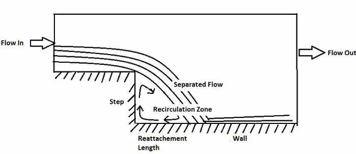
Whenever there is relative movement between a fluid and a solid surface, whether externally round a body, or internally in an enclosed passage, a boundary layer exists with viscous forces present in the layer of fluid close to the surface. Boundary layers can be either laminar or turbulent. A reasonable assessment of whether the boundary layer will be laminar or turbulent can be made by calculating the Reynolds number of the local flow conditions.
Flow separation or boundary layer separation is the detachment of a boundary layer from a surface into a wake. Separation occurs in flow that is slowing down, with pressure increasing, after passing the thickest part of a streamline body or passing through a widening passage, for example. Flowing against an increasing pressure is known as flowing in an adverse pressure gradient. The boundary layer separates when it has travelled far enough in an adverse pressure gradient that the speed of the boundary layer relative to the surface has stopped and reversed direction. The flow becomes detached from the surface, and instead takes the forms of eddies and vortices. The fluid exerts a constant pressure on the surface once it has separated instead of a continually increasing pressure if still attached. In aerodynamics, flow separation results in reduced lift and increased pressure drag, caused by the pressure differential between the front and rear surfaces of the object. It causes buffeting of aircraft structures and control surfaces. In internal passages separation causes stalling and vibrations in machinery blading and increased losses(lower efficiency) in inlets and compressors. Much effort and research has gone into the design of aerodynamic and hydrodynamic surface contours and added features which delay flow separation and keep the flow attached for as long as possible.
Separation and reattachment of turbulent flows occur in many practical engineering applications. It is seen both in internal flow systems such as diffusers, combustors and channels with sudden expansions, and in external flows like flow around airfoil and building. In these situations, the flow experiences an adverse pressure gradient which causes the boundary layer to separate from the solid surface. The flow subsequently reattaches downstream forming a recirculation bubble. The presence of a separated flow, together with a reattaching flow, gives rise to increased unsteadiness, pressure fluctuations which may lead to structure vibrations and noise. The flow over a backward facing step provides an example of above said flow field.
SIMULATION PROCEDURE
- Setting up the case in converge
- Running the simulation in cygwin
- Post convert using cygwin/converge
- Post processing in paraview
The first step is case setup in converge. Open converge and then create the geometry.
We have to create the geometry for backward facing step as shown below:
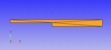
The orientation of normals should be checked such that it should be pointing inwards.
Then run a diagnosis check to find if there are any errors.
If there are no errors, the next step is to name the boundaries.
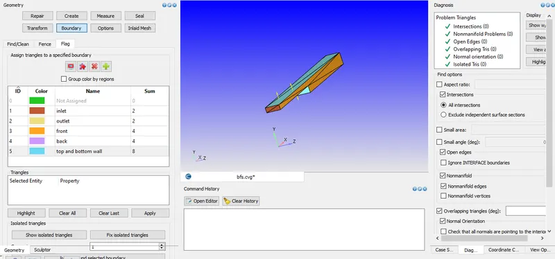
After creating the geometry the next step is to setup the case
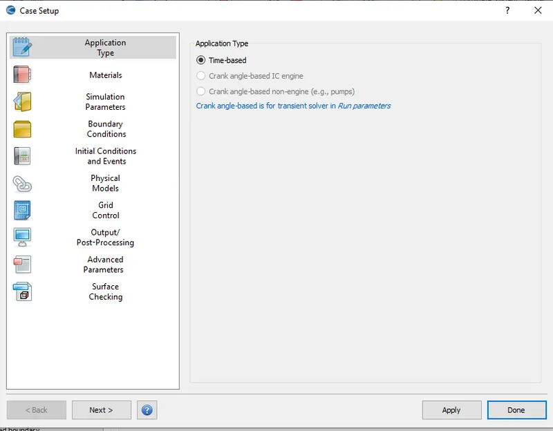
Inorder to run a steady state simulation firstly under application type in the setup tree, a time based simulation must be selected.
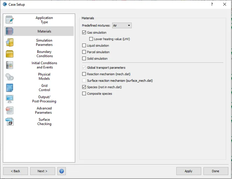
Next in materials, uncheck the reaction mechanism since we are not dealing with any reactions in this problem. In predefined mixtures select air and choose gas simulation. Turn on species.
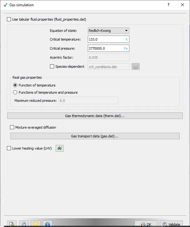
Choose the default properties in the gas simulation.
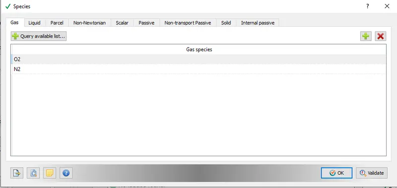
In global transport parameters the default parameters are retained. In species tab, add O2 and N2.
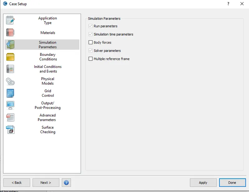
The next one in the case setup tree is the simulation parameters.
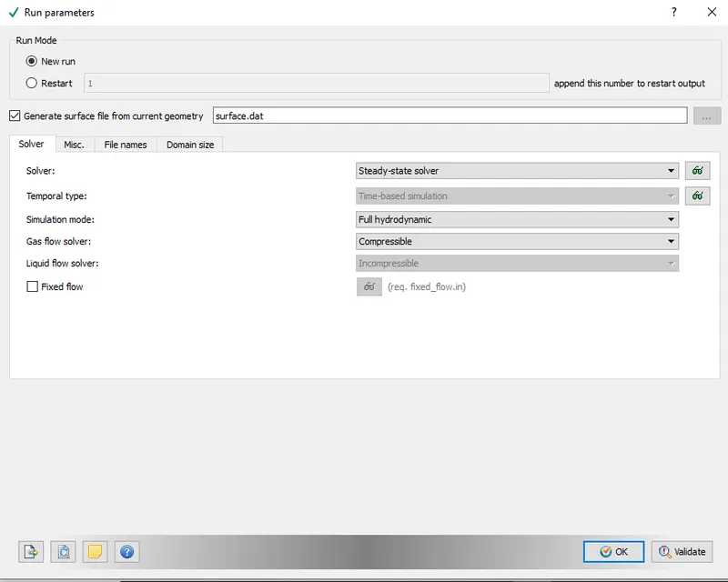
Next in the run parameters tab, select steady state solver. The steady state monitor is a mandatory option for steady state simulations in order to assess convergence of the solution. Turn on steady state monitor. Select the variable to be monitored in the steady state monitor tab. Then select the boundary at which the variable needs to be monitored. Choose oulet because an inlet boundary condition was given.
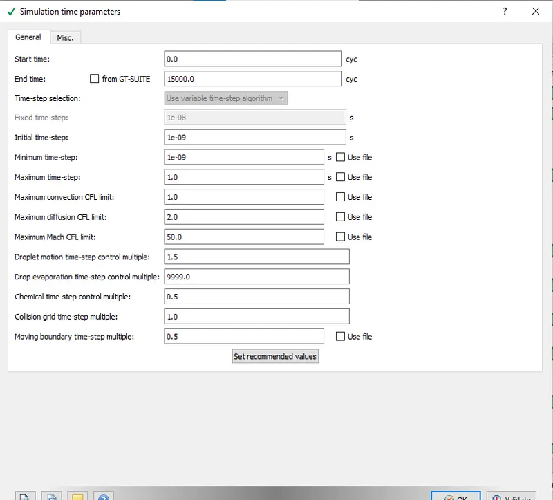
Set the simulation time parameters
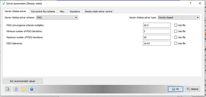
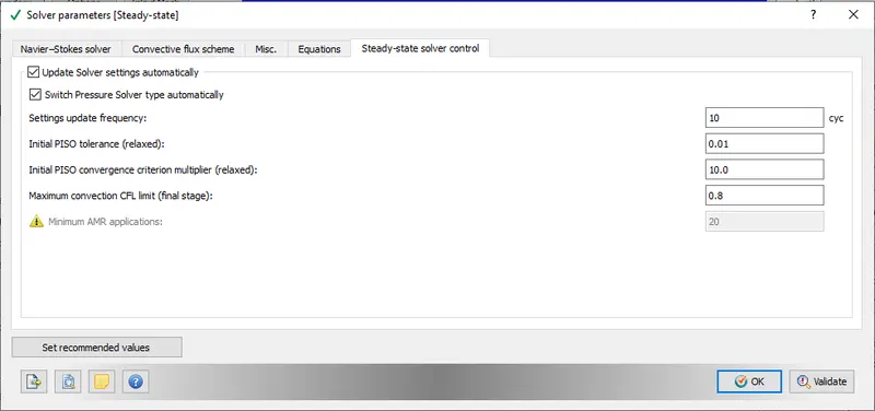
Solver parameters:
Solver scheme - PISO
Solver type - density based
Pressure preconditioner - none
The maximum convection CFL limit should be less than one.
Give the boundary conditions as given below.
For front and back, give the boundary condition as 'TWO_D'.
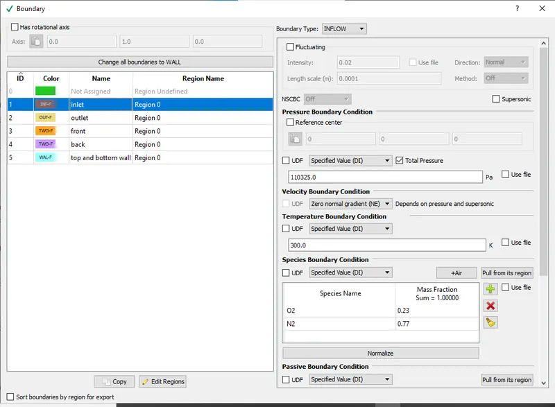
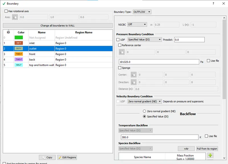
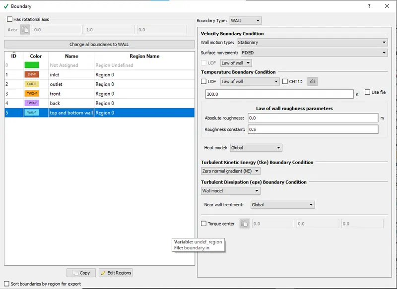
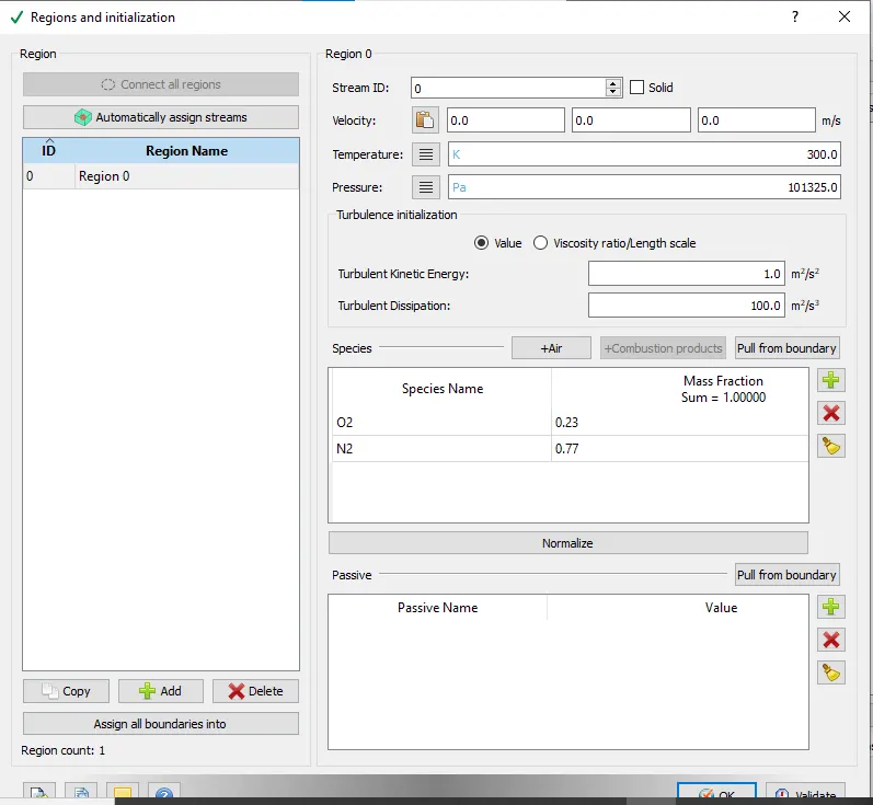
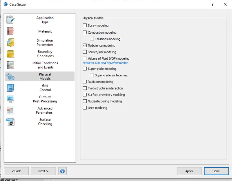
In grid control turn on fixed embedding. In base grid tab, the mesh sizes is to be entered.
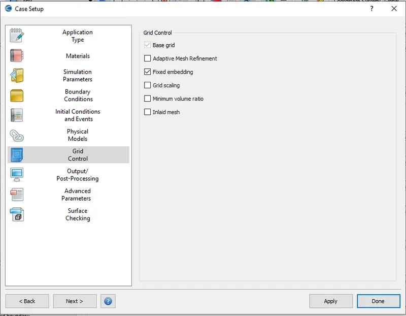
The next step is to provide fixed embedding. Fixed embedding is used to refine the mesh to a value that is lower than the prevalent base size. This is especially useful if we are looking to refine near wall to capture the boundary layer or the wake of a body more accurately. Here fixed embedding is done in top and bottom wall boundary with an embedding scale of one.
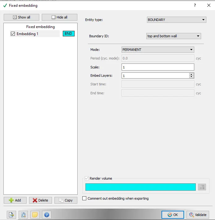
Set the frequency of generation of output files
Once the case setup is completed, export the input files into a required directory. Then launch cygwin and navigate to the directory through CYGWIN in which all input files has been exported and then enter the command to run the simulation ' mpiexec.exe -n 1 converge.exe restricted'. After that post convert using converge and post process the results in paraview.
RESULTS
Case 1
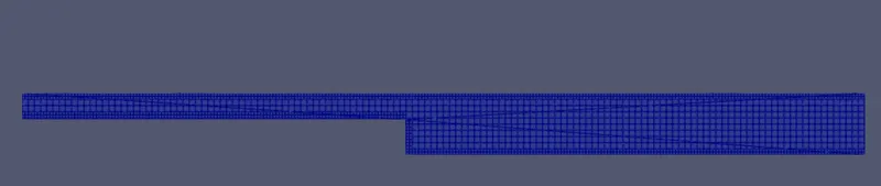
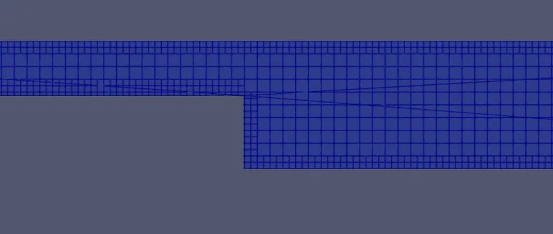
Mesh size ,dx = dy = dz =2e-3m
Mesh
Velocity contour
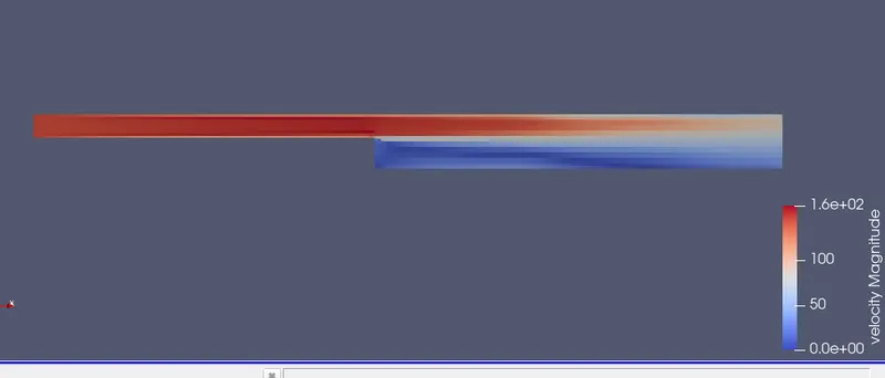
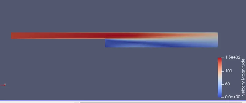
At the inlet the velocity is very high. As the flow proceeds, due to the change in geometry the velocity decreases gradually. The flow separation occurs and the momentum decreases.
Velocity plot
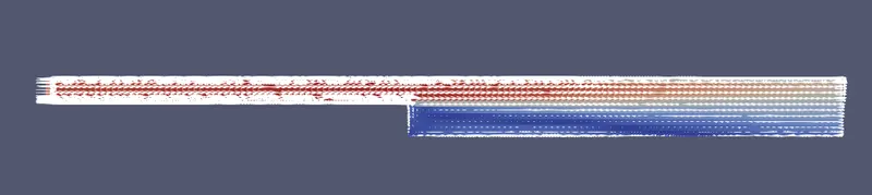
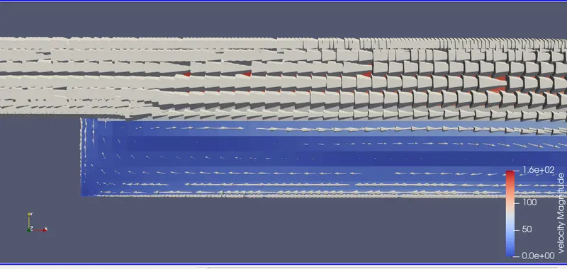
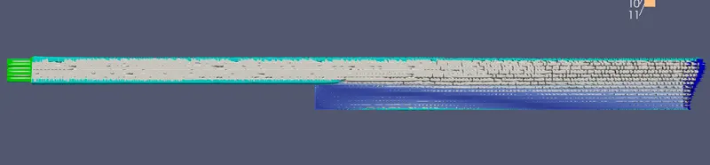
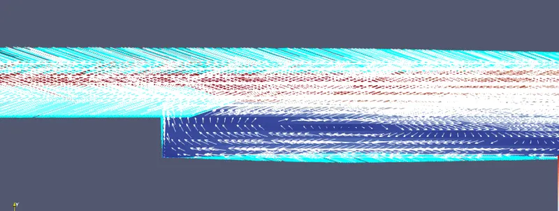
From the vector plots, we can see the recirculation region. When the flow reaches the step, because of expansion of flow channel, pressure gradient exists, it detaches and a recirculation zone is formed. A turbulent boundary layer encounters a sudden back step, causing flow separation. Later the flow eventually reattaches to the bottom wall.
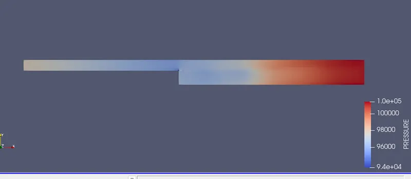
Pressure contour
Mass flow rate
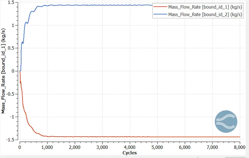
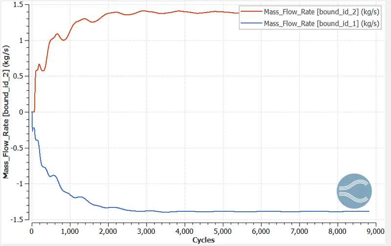
The conservation of mass in this simulation is proved with this plot.
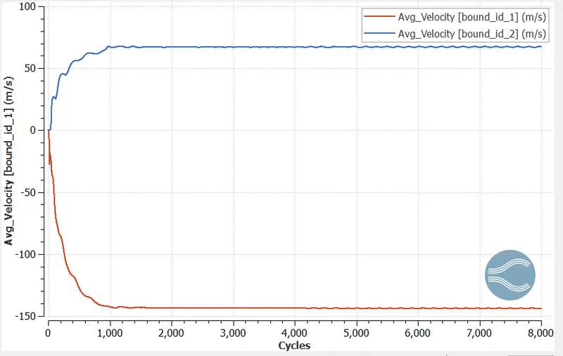
Average velocity
Total pressure
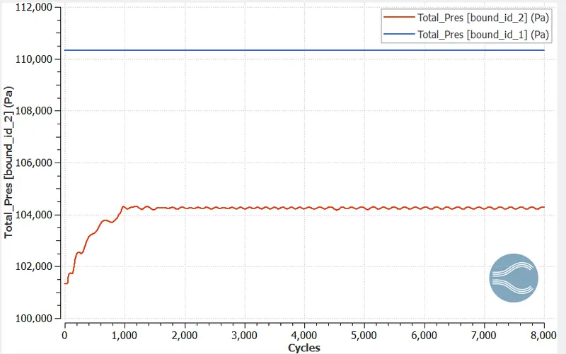
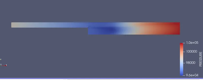
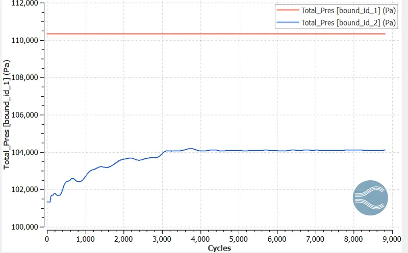
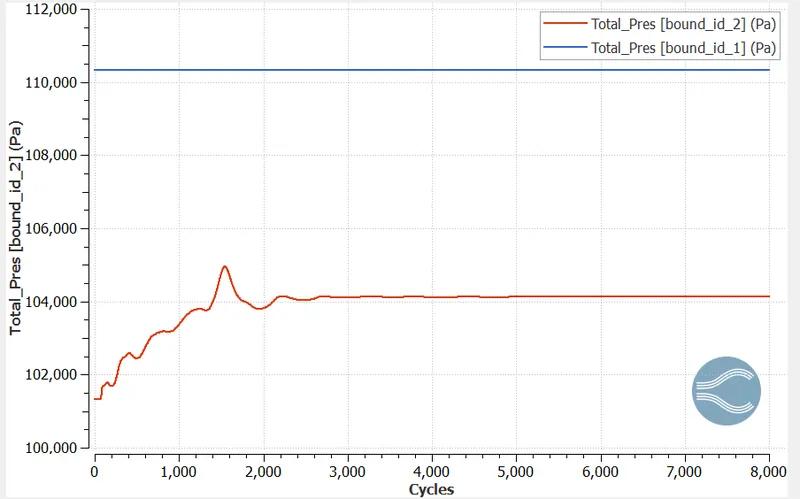
The difference in pressure at inlet and outlet can be seen from this graph.
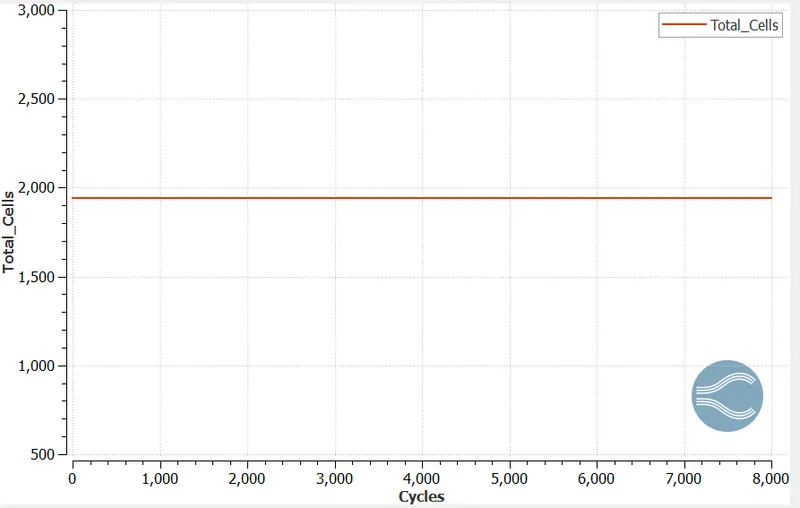
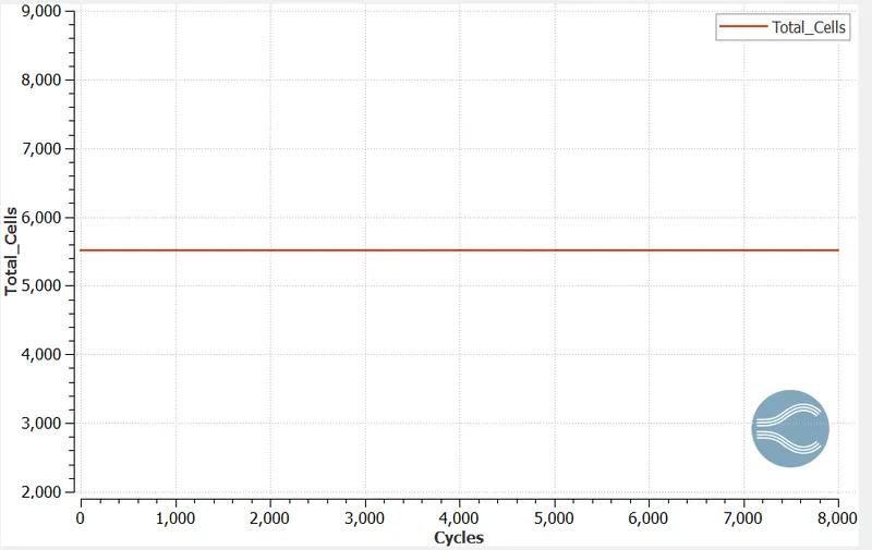
Total cell count
Velocity animation
https://drive.google.com/file/d/1Uw1JeN8QixnkgqSyxUMcJDwrhdQJeAfr/view?usp=sharing
Case 2
Mesh size ,dx = dy = dz =1.5e-3m
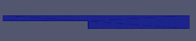
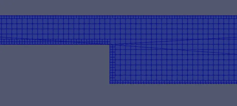
Mesh
Velocity contour
Velocity plot
Pressure contour
Mass flow rate
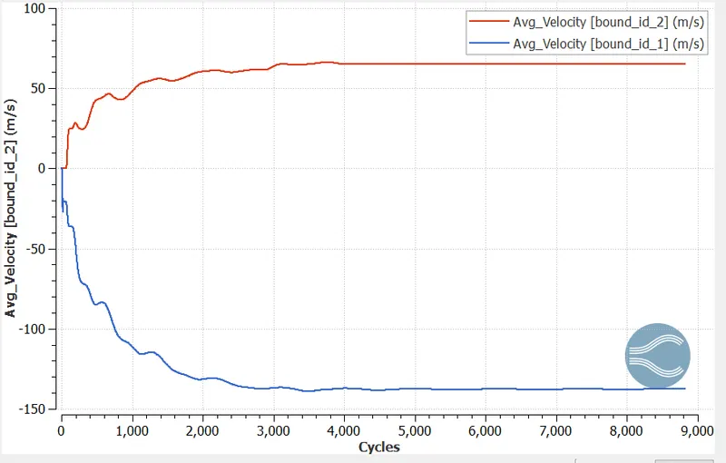
Average velocity
Total pressure
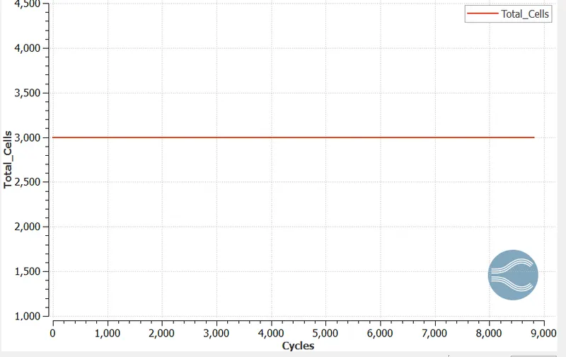
Total cell count
Velocity animation
https://drive.google.com/file/d/1O9sPAcG8wjOeXG-kJQmrarnxwBAuenyx/view?usp=sharing
Case 3
Mesh size ,dx = dy = dz =1e-3m
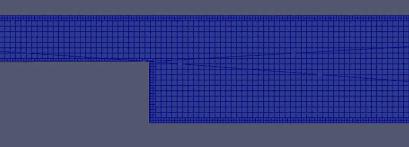
Mesh

Velocity contour
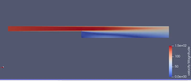
With mesh refinement the the velocity contour is looking more smooth and better.
Velocity plot
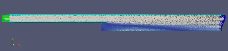
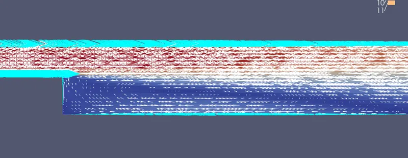
Recirculation zone can be clearly seen in this image.
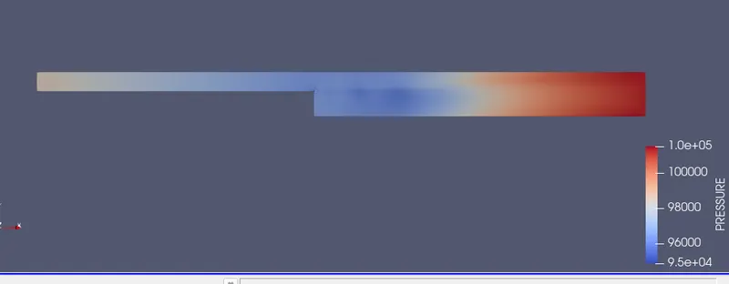
Pressure contour
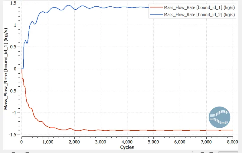
Mass flow rate
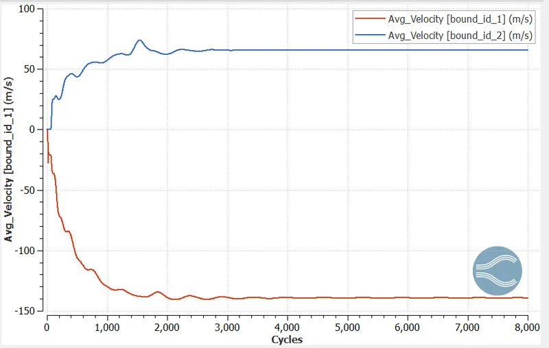
Average velocity
Total pressure
Total cell count
Velocity animation
https://drive.google.com/file/d/1fRW0CgWnWD0gKQwBCzfkynlQJMrwO3kq/view?usp=sharing
From the results of three different mesh sizes we can see that the flow separation occurs as the flow passes through the change in geometry ( step). Flow separation occurs due to the adverse pressure gradient. Flow separation is the most important phenomenon of fluid mechanics because it causes energy loss and deviation of stream lines. The flow becomes detached from the surface, and instead takes the forms of eddies and vortices. The flow separation results in the formation of recirculation zone. The flow reversal is primarily caused by adverse pressure gradient imposed on the boundary layer by the outer potential flow.
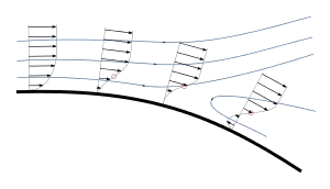
The last profile represents reverse flow which shows separated flow.
CONCLUSION
- Flow over a backward facing step is simulated using converge.
- Flow separation occurs due to the adverse pressure gradient and widening passage.
- The flow separation is caused due to the sudden changes in the geometry. This creates a zone of re-circulation and a point of flow reattachment.
- With mesh refinement computational time and smoothness of results increases.