Week 5.1 - Mid term project - Solving the steady and unsteady 2D heat conduction problem
AIM
1. Steady state analysis & Transient State Analysis
Solve the 2D heat conduction equation by using the point iterative techniques. The Boundary conditions for the problem are as follows;
Top Boundary = 600 K
Bottom Boundary = 900 K
Left Boundary = 400 K
Right Boundary = 800 K
You will implement the following methods for solving implicit equations.
1. Jacobi
2. Gauss-seidel
3. Successive over-relaxation
absolute error criteria is 1e-4
2. Write code for both implicit and explicit schemes (This is for the Transient Analysis only)
3. Write a detailed explanation for your results, plots or codes
Theory
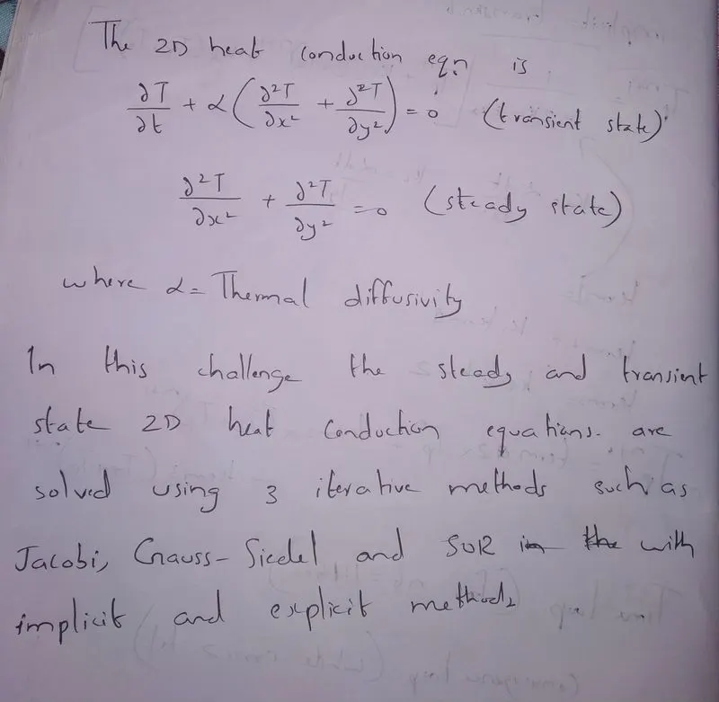
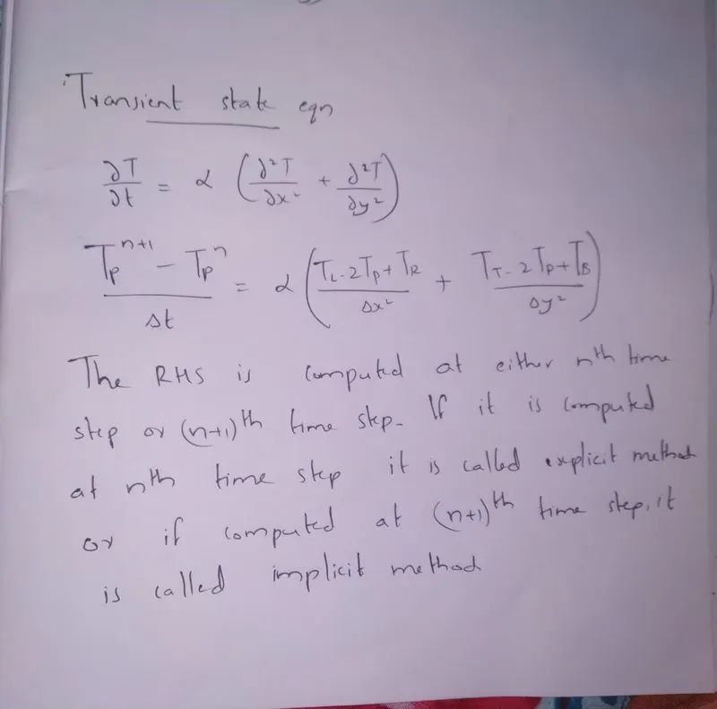
Explicit and implicit methods are approaches used in numerical analysis for obtaining numerical approximations to the solutions of time-dependent ordinary and partial differential equations, as is required in computer simulations of physical processes. Explicit methods calculate the state of a system at a later time from the state of the system at the current time, while implicit methods find a solution by solving an equation involving both the current state of the system and the later one.
Implicit methods require an extra computation, and they can be much harder to implement. Implicit methods are used because many problems arising in practice are stiff, for which the use of an explicit method requires impractically small time steps to keep the error in the result bounded. For such problems, to achieve given accuracy, it takes much less computational time to use an implicit method with larger time steps.
Iterative methods
The approximate methods for solving system of linear equations makes it possible to obtain the values of the roots system with the specified accuracy. This process of constructing such a sequence is known as iteration. Three closely related method studied in this work are all iterative in nature. Unlike the direct methods, which attempts to calculate an exact solution in a finite number of operations, these methods starts with an initial approximation and generate successively improved approximations in an infinite sequence whose limit is the exact solution. In practical terms, this has more advantage, because the direct solution will be subject to rounding errors.
Jacobi method
In numerical linear algebra, the Jacobi method is an algorithm for determining the solutions of a
diagonally dominant system of linear equations. Each diagonal element is solved for, and an approximate value is plugged in. The process is then iterated until it converges. This algorithm is a stripped- down version of the Jacobi transformation method of matrix diagonalization. In the Jacobi method, all of the values of the unknowns are updated before any of the new information
is used in the calculations.
Gauss Siedel method
In numerical linear algebra, the Gauss–Seidel method, also known as the Liebmann method or the method of successive displacement, is an iterative method used to solve a system of linear equations. Though it can be applied to any matrix with non-zero elements on the diagonals, convergence is only guaranteed if the matrix is either strictly diagonally dominant, or symmetric and positive definite.
Successive Over Relaxation (SOR) method
In numerical linear algebra, the method of successive over-relaxation (SOR) is a variant of the Gauss-Seidel method for solving a system of linear equations, resulting in faster convergence. A similar method can be used for any slowly converging iterative process. The successive over-relaxation (SOR), is devised by applying extrapolation to the Gauss-Seidel method.
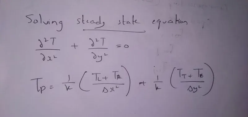
Solving the steady state 2D heat conduction equation
Main code
%solving the 2D steady state heat conduction equations
clear all
close all
clc

%no. of nodes
nx=10;
ny=nx;

x=linspace(0,1,nx);
y=linspace(0,1,ny);

dx=x(2)-x(1);
dy=y(2)-y(1);

[xx,yy]=meshgrid(x,y); %creating mesh

%initial and boundary conditions
T=300*ones(nx,ny);

T(1,2:nx-1)=600; %Top Boundary
T(nx,2:nx-1)=900; %Bottom Boundary
T(2:nx-1,1)=400; %Left Boundary
T(2:nx-1,nx)=800; %Right Boundary

%Calulcating temperatures at corners
T(1,1)=(600+400)/2;
T(1,10)=(600+800)/2;
T(10,1)=(400+900)/2;
T(10,10)=(900+800)/2;

Told=T;
%defining error and tolerance
error=9e9;
tol=1e-4;

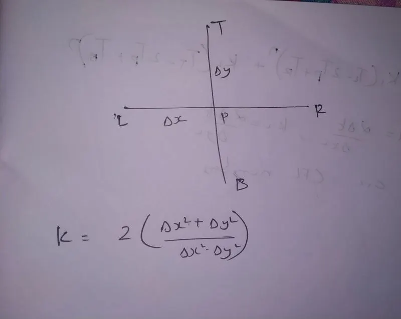
k=2*((dx^2+dy^2)/((dx^2)*(dy^2)));


   T_jacobi = jacobi_iter(error,tol,nx,ny,xx,yy,T,k,Told,dx,dy);


   T_gauss = gauss_iter(error,tol,nx,ny,xx,yy,T,k,Told,dx,dy);

   T_sor = sor(error,tol,nx,ny,xx,yy,T,k,Told,dx,dy)
Function code - Jacobi iteration
function T = jacobi_iter(error,tol,nx,ny,xx,yy,T,k,Told,dx,dy)


jacobi_iter=1;

while(error>tol)

    for i =2:nx-1
        for j=2:ny-1
            term1 = (Told(i-1,j)+Told(i+1,j))/(k*(dx^2));
            term2 = (Told(i,j-1)+Told(i,j+1))/(k*(dy^2));
            T(i,j)=term1 + term2;
        end
    end

    error=max(max(abs(Told-T)));
    Told=T;
    jacobi_iter=jacobi_iter+1;

    figure(1)
    colormap(jet)
    colorbar
    [c,d]=contourf(xx,yy,T);
    clabel(c,d);
    set(gca,'YDIR','reverse')
    title_text=sprintf('iteration number= %d',jacobi_iter);
    title(title_text);
    xlabel('X-axis')
    ylabel('Y-axis')
end
Function code - Gauss Siedel iteration
function T = gauss_iter(error,tol,nx,ny,xx,yy,T,k,Told,dx,dy)


gauss_iter=1;

while(error>tol)

    for i =2:nx-1
        for j=2:ny-1
            term1 = (T(i-1,j)+Told(i+1,j))/(k*(dx^2));
            term2 = (T(i,j-1)+Told(i,j+1))/(k*(dy^2));
            T(i,j)=term1 + term2;
        end
    end

    error=max(max(abs(Told-T)));
    Told=T;
    gauss_iter=gauss_iter+1;

    figure(2)
    colormap(jet)
    colorbar
    [c,d]=contourf(xx,yy,T);
    clabel(c,d);
    set(gca,'YDIR','reverse')
    title_text=sprintf('iteration number= %d',gauss_iter);
    title(title_text);
    xlabel('X-axis')
    ylabel('Y-axis')
end
Function code - SOR iteration
function T = sor(error,tol,nx,ny,xx,yy,T,k,Told,dx,dy)


sor=1;
omega=1.2;
% absolute error criteria > tolerance
while(error>tol)

    for i =2:nx-1
        for j=2:ny-1
           Tgauss = (T(i-1,j)+Told(i+1,j))/(k*(dx^2))+(T(i,j-1)+Told(i,j+1))/(k*(dy^2));

            T(i,j) = (1-omega)*(Told(i,j)) + omega*Tgauss
        end
    end

    error=max(max(abs(Told-T)));
    Told=T;
    sor=sor+1;

    figure(3)
    colormap(jet)
    colorbar
    [c,d]=contourf(xx,yy,T);
    clabel(c,d);
    set(gca,'YDIR','reverse')
    title_text=sprintf('iteration number= %d',sor);
    title(title_text);
    xlabel('X-axis')
    ylabel('Y-axis')
end
Code explanation
- Inputs are given
- Mesh grid is created
- Initial and boundary conditions are given
- Temperature at the corners are calculated
- Error and tolerance is defined, the value of constant k is also defined
- Function code for different iterations is created, later they are called into the main code
- In the function code, error is calculated and the loop will run till the error values becomes less than the tolreance value.
- In the code for plotting, colormap sets the colormap for the current figure to one of the predefined colormaps, colorbar display the current colormap and indicate the mapping of data values into the colormap and contourf(xx,yy,T) creates a filled contour plot.
Results - steady state
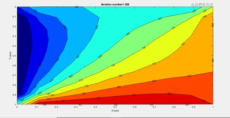
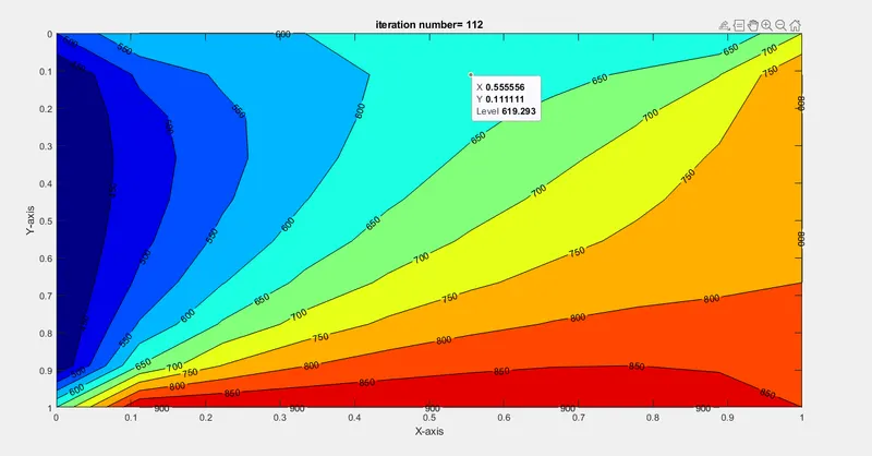
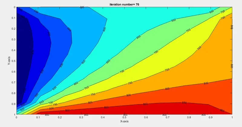
From the above 3 plots, it is clear that SOR method takes less number of iterations compared to the other methods. SOR method converges faster.
Solving the transient state 2D heat conduction equation
Explicitly
Code with explanation
%solving the 2D transient state heat conduction equations explicitly
clear all
close all
clc

%no. of nodes
nx=10;
ny=nx;

x=linspace(0,1,nx);
y=linspace(0,1,ny);

dx=x(2)-x(1);
dy=y(2)-y(1);
dt=0.001;


[xx,yy]=meshgrid(x,y); %creating mesh

%initial and boundary conditions
T=300*ones(nx,ny);

T(1,2:nx-1)=600; %Top Boundary
T(nx,2:nx-1)=900; %Bottom Boundary
T(2:nx-1,1)=400; %Left Boundary
T(2:nx-1,nx)=800; %Right Boundary

%Calulcating temperatures at corners
T(1,1)=(600+400)/2;
T(1,10)=(600+800)/2;
T(10,1)=(400+900)/2;
T(10,10)=(900+800)/2;

Told=T;
%defining error and tolerance
error=9e9;
tol=1e-4;

alpha=1.5;
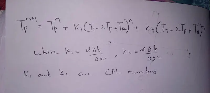
k1=alpha*(dt/dx^2);
k2=alpha*(dt/dy^2);
CFL=k1+k2 %to find the CFL number

  for k=1:1400 %no. of iteration

    for i =2:nx-1
        for j=2:ny-1
            term1 = Told(i,j);
            term2 = k1*(Told(i-1,j)-2*Told(i,j)+Told(i+1,j));
            term3 = k2*(Told(i,j-1)-2*Told(i,j)+Told(i,j+1));
            T(i,j)=term1 + term2 + term3;
        end
    end

    error=max(max(abs(Told-T)));%to find the error
    Told=T;%updating values


    figure(1)
    colormap(jet) %sets the colormap for the current figure to one of the predefined colormaps
    colorbar % Colorbars display the current colormap and indicate the mapping of data values into the colormap
    [c,d]=contourf(xx,yy,T); % creates a filled contour plot
    clabel(c,d);
    set(gca,'YDIR','reverse')% to reverse the y direction in the plot
    xlabel('X-axis') %labelling the axis
    ylabel('Y-axis')

  end
Results (Transient state_explicit)
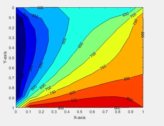
Solving the transient state 2D heat conduction equation(implicitly)
Main code
%solving the 2D transient state heat conduction equations implicitly
clear all
close all
clc

%no. of nodes
nx=10;
ny=nx;

x=linspace(0,1,nx);
y=linspace(0,1,ny);

dx=x(2)-x(1);
dy=y(2)-y(1);
dt=0.01;


[xx,yy]=meshgrid(x,y); %creating mesh

%initial and boundary conditions
T=300*ones(nx,ny);

T(1,2:nx-1)=600; %Top Boundary
T(nx,2:nx-1)=900; %Bottom Boundary
T(2:nx-1,1)=400; %Left Boundary
T(2:nx-1,nx)=800; %Right Boundary

%Calulcating temperatures at corners
T(1,1)=(600+400)/2;
T(1,10)=(600+800)/2;
T(10,1)=(400+900)/2;
T(10,10)=(900+800)/2;

Told=T;
T_prev=Told;
%defining error and tolerance
error=9e9;
tol=1e-4;

alpha=1.5;
k1=alpha*(dt/dx^2);
k2=alpha*(dt/dy^2);


T_implicit_jacobi= jacobi_iter_implicit(error,tol,nx,ny,xx,yy,T,Told,T_prev,dx,dy,dt,alpha,k1,k2);

T_implicit_gauss = gauss_iter_implicit(error,tol,nx,ny,xx,yy,T,Told,T_prev,dx,dy,dt,alpha,k1,k2);

 T_implicit_sor = sor_implicit(error,tol,nx,ny,xx,yy,T,Told,T_prev,dx,dy,dt,alpha,k1,k2);
Function code-Jacobi iteration
function T = jacobi_iter_implicit(error,tol,nx,ny,xx,yy,T,Told,T_prev,dx,dy,dt,alpha,k1,k2)


jacobi_iter=1;


for k=1:1400
    error=9e9;
    while(error>tol)
        for i =2:nx-1
            for j=2:ny-1
                term1 = (1+(2*k1)+(2*k2))^-1;
                term2 = k1*term1;
                term3 = k2*term1;
                H = (Told(i-1,j)+Told(i+1,j));
                V = (Told(i,j-1)+Told(i,j+1));
                T(i,j)=(T_prev(i,j)*term1) + (H*term2) + (V*term3);
            end
        end

        error=max(max(abs(Told-T)));
        Told=T;
        jacobi_iter=jacobi_iter+1;
    end
    T_prev=T;
end
figure(1)
colormap(jet) %sets the colormap for the current figure to one of the predefined colormaps
colorbar% Colorbars display the current colormap and indicate the mapping of data values into the colormap
[c,d]=contourf(xx,yy,T);% creates a filled contour plot
clabel(c,d);
set(gca,'YDIR','reverse')
title_text=sprintf('iteration number= %d',jacobi_iter);
title(title_text);
xlabel('X-axis')
ylabel('Y-axis')
end
Function code-Gauss siedel iteration
function T = gauss_iter_implicit(error,tol,nx,ny,xx,yy,T,Told,T_prev,dx,dy,dt,alpha,k1,k2)


gauss_iter_impli=1;


for k=1:1400
    error=9e9;
    while(error>tol)
        for i =2:nx-1
            for j=2:ny-1
                term1 = (1+(2*k1)+(2*k2))^-1;
                term2 = k1*term1;
                term3 = k2*term1;
                H = (T(i-1,j)+Told(i+1,j));
                V = (T(i,j-1)+Told(i,j+1));
                T(i,j)=(T_prev(i,j)*term1) + (H*term2) + (V*term3);
            end
        end

        error=max(max(abs(Told-T)));
        Told=T;
        gauss_iter_impli=gauss_iter_impli+1;
    end
    T_prev=T;
end
figure(2)
colormap(jet)
colorbar
[c,d]=contourf(xx,yy,T);
clabel(c,d);
set(gca,'YDIR','reverse')
title_text=sprintf('iteration number= %d',gauss_iter_impli);
title(title_text);
xlabel('X-axis')
ylabel('Y-axis')
end
Function code-SOR iteration
function T = sor_implicit(error,tol,nx,ny,xx,yy,T,Told,T_prev,dx,dy,dt,alpha,k1,k2)


sor_implicit=1;
omega = 1.2;

for k=1:1400
    error=9e9;
    while(error>tol)
        for i =2:nx-1
            for j=2:ny-1
                term1 = (1+(2*k1)+(2*k2))^-1;
                term2 = k1*term1;
                term3 = k2*term1;
                H = (T(i-1,j)+Told(i+1,j));
                V = (T(i,j-1)+Told(i,j+1));
                T_gauss(i,j)=(T_prev(i,j)*term1) + (H*term2) + (V*term3);
                T(i,j)=((1-omega)*Told(i,j))+omega*T_gauss(i,j);

            end
        end

        error=max(max(abs(Told-T)));
        Told=T;
        sor_implicit=sor_implicit+1;
    end
    T_prev=T;
end
figure(3)
colormap(jet)
colorbar
[c,d]=contourf(xx,yy,T);
clabel(c,d);
set(gca,'YDIR','reverse')
title_text=sprintf('iteration number= %d',sor_implicit);
title(title_text);
xlabel('X-axis')
ylabel('Y-axis')
end
Results (Transient state_implicit)
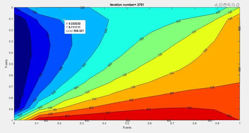
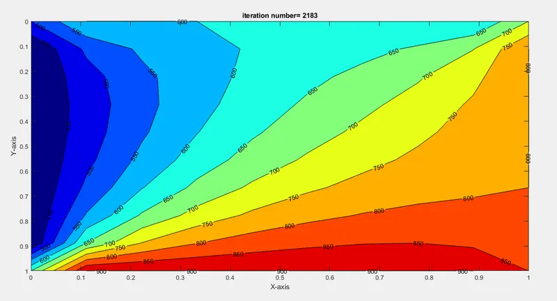
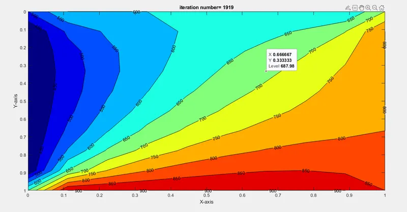
From the above 3 plots, it is clear that SOR method takes less number of iterations compared to the other methods. SOR method converges faster.
Conclusions
While solving the steady state and transient state equations, it is proved that steady state equations takes lesser number of iterations compared to transient state.
In both schemes SOR method converges faster compared to jacobi and gauss siedel methods.
In tranisent state while solving implicitly and explicitly, the explicit method solves faster.